Contemporary Challenges: Fall-2023
Homework 6 (SOLUTION): Due Day 29 Monday 12/1

1. Cosmic Background Radiation S1 4748S

   The universe is filled with thermal radiation that has a blackbody spectrum at an effective temperature of 2.7 K. What is the wavelength of light that corresponds to the peak in \(S_\lambda\) (\(S_\lambda\) is the spectral distribution with respect to wavelength)? In what region of the electromagnetic spectrum is this peak wavelength?

   The peak wavelength of a blackbody spectrum depends on temperature, following the relationship \(\lambda _{\text{max} }=hc/(4.96k_B T)\). This is sometimes refered to as Wien's displacement law. The order of magnitude, \(\lambda _{\text{max}} \approx hc/(k_B T)\), can be estimated by noting that the strongest light emission will come from the highest frequency oscillators, with the caveat that photon energy won't go much beyond \(k_B T\). The precise numerical factor, 4.96, can be found by differentiating Planck's law with respect to wavelength to find the maximum.

   For a temperature of \(2.7 \text{ K}\) the peak wavelength is \(\lambda_{\max }=1.1 \text{ mm}\). This in the microwave region of the EM spectrum, which is why this is often called the cosmic microwave background radiation. The boundary between microwaves, high frequency radio waves, terahertz, and far-IR light are not well defined. It could be argued to be in any of these regions, but it's most commonly associated with microwaves.

2. Efficiency of a solar cell S1 4748S
   

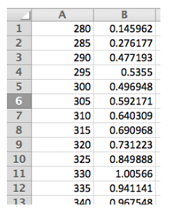
   Download the file extraterr_solar.csv, which is in comma-separated-variable (csv) format. Open the csv file in a spreadsheet program such as Excel. The data is the spectral intensity with respect to wavelength, \(S_\lambda\), for the sunlight that is hitting a satellite above the earth. The first column is wavelength in units of nanometers. The second column is spectral intensity in units of W/(m\(^2\cdot\)nm).

   1. Use a spreadsheet to perform a simple numerical integration (Riemann sum) to find the total energy flux hitting the satellite. Explain your method using summation notation. Additionally, write down the formula you enter in the spreadsheet (e.g. =SUM(B1:B745)). Give your final answer in units of W/m\(^2\) and check that it is reasonable.

      The numerical integration is performing \(\sum_{i=1}^{N} I_{\lambda, i} \cdot \Delta \lambda\) where \(I_{\lambda, i}\) is the \(i^{\text { th }}\) value of spectral intensity and \(\Delta \lambda=5\) nm. In Excel I used the formula =5*SUM(B1:B745). Performing this sum yields a total energy flux of \(I=1348 \frac{\mathrm{W}}{\mathrm{m}^{2}}.\)

   2. Consider a narrow band of wavelengths, from 552.5 nm to 557.5 nm. (The bandwidth is 5 nm and the central wavelength is 555 nm). All the photons in this bandwidth have very similar energy, \(E_{\text{photon}} \approx\) (1240 nm\(\cdot\)eV)/(555 nm). How many photons per second per \(\text{m}^2\) are in this spectral band of sunlight? Explain your method using standard mathmeatical notation. Additionally, write down the formula that you entered into the spreadsheet.

      The spectral intensity at 555 \(\mathrm{nm}\) is 1.86\(\frac{\mathrm{W}}{\mathrm{nm\cdot m}^{2}}\) and the photon energy is 2.23 \(\mathrm{eV}\). Multiplying the spectral intensity by the 5 nm spectral width and dividing by the photon energy gives a photon flux of \(I_{\mathrm{ph}}=2.6 \times 10^{19} \frac{\text { photons }}{\mathrm{s} \cdot \mathrm{m}^{2}}\). In Excel I used the formula =5*B56/(1.6E-19*1240/A56)

      The calculation that you did for part b can now be applied to every row in your spreadsheet. You will need these numbers for part c.
      

   3. Silicon solar cells absorb photons if \(E_{\text{photon}}> 1.1\text{ eV}\). That is to say, \(E_{\text{photon}}\) must be greater than gap between occupied and unoccupied quantum energy levels in silicon. Use your spreadsheet to calculate how many photons per second per \(\text{m}^2\) have sufficient energy to be absorbed by a solar cell. Write down the formula that you entered into the spreadsheet.

      In my spreadsheet I created column C which lists the number of photons in each spectral bin. I summed the photon numbers in these spectral bins, starting at a photon energy of 1.1 eV and going up to the highest photon energy (around 4.3 eV). In Excel I used the formula =SUM(C1:C170). The result is \(3.38 \times 10^{21} \frac{\text { photons }}{\mathrm{s} \cdot \mathrm{m}^{2}}\).

   4. The electrical energy produced by a silicon solar cell cannot exceed \((1.1\text{ eV})\ \times\text{ (number of absorbed photons)}\). Calculate the maximum possible rate that electrical energy could be produced by a solar cell attached to this satellite per unit area. Give your answer in units of \(\text{W/m}^2\).

      The power per area generated by the silicon solar cell is the total photon flux above the 1.1 eV cutoff (the result from part d) multiplied by the energy that can be harvested from each photon which is \(1.1 \mathrm{eV}=1.76 \times 10^{-19} \mathrm{J}\). Performing this calculation yields a total power per area of \(596 \frac{\mathrm{W}}{\mathrm{m}^{2}}.\)

   5. Compare your answers to part a and part d. What is the maximum possible efficiency of the solar cell (i.e. the ratio of the electrical energy output to the total energy input)?

      The ratio of the power per area found in part e) to the intensity of sunlight found in part a) is 44\(\%\). The rest of the sun's energy is either not absorbed, \(24\%\), or turned into heat inside the silicon, \(32\%\).
      
      This homework question is a coarse-grained model that respects the basic operating principle of a solar cell. However, it is not the complete story. The true efficiency limit for a solar cell made from a single pn junction, operating with natural solar intensity is about 33%.

      To understand this fully, we should study the physics of pn junctions. Then we would know the max volage we could expect from the solar cell (it is slightly less than the bandgap voltage). We would also know how much current we could extract without drastically diminishing the voltage. (The current must be slightly smaller than 1 electron per absorbed photon).

      Shockley & Queisser published such calculations in 1961. The paper is 10 pages long. On page 3 they present a zeroth-order estimate, which is consistent with this homework question: \begin{align} &\text{``ultimate efficiency''}\notag\\ &=x_g\left(\int_{x_g}^{\infty}\frac{x^2\ dx}{e^x - 1}\right)/\left(\int_0^{\infty}\frac{x^3\ dx}{e^x -1}\right) \end{align} where \(x_g = E_{gap}/(k_\text{B} T_{sun})\) and \(T_{sun} \approx 6000\text{ K}\). The integrands in this equation come from Planck's law. The maximum efficiency, \(44\%\), occurs at \(E_{gap} = 1.1\text{ eV}\). The next 7 pages of Shockley & Queisser's paper considers the details of a real pn junction, with the fundamental limitations of working at room temperature with a limited intensity of solar radiation. They arrived at a limit of 33%.

3. Reentry Heating of the Space Shuttle S1 4748S

   When NASA's Space Shuttle Orbiter descends from orbit it must pass through the upper reaches of Earth's atmosphere where the air is extremely thin. In this upper atmosphere, air molecules collide with the space shuttle and cause significant heating (transfer of kinetic energy). At very high altitudes, there aren't enough air molecules for convective heat transport. At these altitudes, the primary mechanism for cooling the Orbiter is the emission of blackbody radiation.

   The Orbiter has a heat shield on its underside (see the black panels in the photo at the bottom of the page). This heat shield reaches a temperature of 2000 K. The topside of the Orbiter stays cool (\(\approx\) 300 K).

   

   Estimate the maximum rate of decent of the shuttle through the upper atmosphere (the decrease in elevation per unit time). The primary constraint is that the temperature of the heat shield cannot safely exceed 2000 K (glowing red hot). This estimate will require a few steps:

   1. At what rate is blackbody radiation emitted from the Orbiter's heat shield when its underside reaches a temperature of 2000 K? Give your answer in J/s.

      Note: the space shuttle is about 35 m long, and has a wingspan (from wingtip to wingtip) of 25 m.

      We want to know the rate that energy is radiated from the bottom of the space shuttle when it is at \(T=2000\text{ K}\). The surface area is approimately \((35\times25)/2\text{ m}^2\). The thermal radiation emission rate is \begin{align} \sigma T^4 [440\text{ m}^2] = (5.7\times10^{-8}\text{ J/s}\cdot \text{K}^4)(2000\text{ K})^4(440\text{ m}^2) = 5\times10^8\text{ J/s} \end{align}

   2. The Orbiter has a velocity component parallel to the Earth's surface, \(v_\parallel\), and a velocity component pointing toward the Earth's surface, \(v_\perp\). To build physical intuition about the descent, let's use reasoning and simple modeling to test some hypotheses about the dominant energy transformations involved. As a first hypothesis, we'll consider a plausible coarse-grained model: assume the Orbiter's total kinetic energy remains constant during reentry, while its gravitational potential energy decreases. Apply the First Law of Thermodynamics (conservation of energy) to estimate the maximum value of \(v_\perp\). Express your answer in units of m/s.

      Note: Gravitational potential energy is changing, and electromagnetic radiation energy is being generated. The orbiter's mass is about 80,000 kg, similar to the mass of 80 cars.

      If the change in K.E. is negligible, then \(m g \Delta h/\Delta t \le 5\times 10^8\text{ J/s}\), where \(m g \Delta h/\Delta t\) is the rate of change of gravitational potential energy. \begin{align} \frac{\Delta h}{\Delta t} &\le \frac{5\times10^8\text{ J/s}}{(10^5\text{ kg})(10\text{ ms}^{-2})}\\ &\le 500\text{ m/s} \end{align}

   3. Now try analyzing the descent again, this time accounting for the changing kinetic energy of the Orbiter. Use the following information to construct a plausible coarse-grained model. As before, we're using physical reasoning to test hypotheses about the descent, but now incorporating additional detail to better reflect the energy transformations involved. Our goal is to estimate the time required for a safe descent:

      Time of ignition for the de-orbit burn is about 60 minutes before landing. The burn lasts 3 to 4 minutes and slows the Orbiter enough to begin its descent. About 30 minutes before landing, the Orbiter begins to encounter the effects of the upper atmosphere and the heat shields start to heat up. This usually occurs at an altitude of about 130 km, more than 8,000 km from the landing site. At this point, the Orbiter is traveling at 7500 m/s relative to the atmosphere. Around 15 minutes before landing, it has descended to an altitude of about 10 km (comparable to the cruising altitude of commercial aircraft) and is traveling at approximately the speed of sound (340 m/s).

      Using this new information about changes in velocity and altitude, estimate the time required for “braking with fire” (the hot and fiery segment of the descent). Compare to the actual timeline. What physical mechanisms are still missing from the coarse-grained model of the fiery descent? What would be a sensible next level of model refinement?

      \begin{align} \text{Initial KE} &= \frac{1}{2} m v^2 = \frac{1}{2}(10^5\text{ kg})(7500\text{ m/s})^2\\ &\qquad \qquad= 3\times 10^{12}\text{ J}\\ \text{Final KE} &= \frac{1}{2}(10^5\text{ kg})(340\text{ m/s})^2 = 5\times10^9\text{ J} \end{align} Compare these numbers to the change in gravitational potential energy \begin{align} \Delta U_g &= m g \Delta h\\ &=(10^5\text{ kg})(10\text{ m s}^{-2})(1.2\times10^5\text{ m})\\ &= 1.2\times10^{11} \text{ J} \end{align} This shows that the shuttle must lose much more K.E. than gravitational potential energy. If the K.E. is lost at a rate of \(5\times10^8\text{ J/s}\), the space shuttle descent would take \begin{align} \Delta t = \frac{3\times10^{12}\text{ J}}{5\times10^8\text{ J/s}} &= 0.6\times10^4\text{ s}\\ & = 6000\text{ s}\\ & = 100\text{ minutes} \end{align} This time is longer than 15 minute.

      There must be something wrong with my assumptions. For a more refined description, I should consider the possibility of transferring kinetic energy to the “wind trail” behind the orbiter, especially when the atmosphere gets thicker.

      We could also consider the thermal conductivity of the atmosphere, which would provide an additional mechanism for heat energy to be dissipated.

4. Two-layer model for estimating the Earth's temperature S1 4748S Two layers of plexiglass are surrounding the Earth. One layer is 5 km above sea level, the other layer is 10 km above sea level. These plexiglass layers have replaced the gaseous atmosphere. Both layers of plexiglass are transparent to the solar spectrum (wavelengths centered around 500 nm), but fully absorb the thermal radiation emitted from the surface of the Earth. The surface of the Earth absorbs \(70\%\) of the incident sunlight and reflects the rest. Assume that the Earth distributes the absorbed solar energy uniformly across its spherical surface, therefore, it has a uniform temperature, \(T_{\text{surf}}\). Every part of this system is in steady state, meaning, all temperatures are stable.
   1. Draw an energy flow diagram for this system with three boxes representing (i) the surface of the Earth, (ii) the first plexiglass layer, (iii) the second plexiglass layer. Draw arrows to represent energy transported by short-wavelength light (solar radiation centered around 500 nm) and long-wavelength light (earth glow centered around 10,000 nm). If energy is being exchanged in two directions, show this with two separate arrows.

      

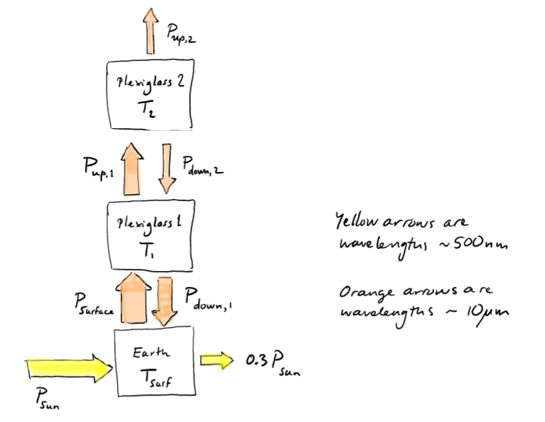
   2. The surface of the earth has temperature \(T_{\text{surf}}\), the first plexiglass layer has temperature \(T_1\), and the second plexiglass layer has temperature \(T_2\). Treat these as unknowns (we will determine them in part c). Use the idea of balanced energy rates to write down a set of mathematical relationships relating \(T_{\text{surf}}\), \(T_1\) and \(T_2\). Other parameters that may appear in your expressions include:
      \(\quad I_{\text{sun}}\), intensity of sunlight
      \(\quad R_{\text{earth}}\), radius of Earth
      \(\quad \sigma\), the Stefan-Boltzmann constant
      
      Note: Remember that the absorption of Sunlight depends on the size of the earth's shadow, not on the surface area of the earth.
      Note: The surface area of the plexiglass layers are almost equal to the surface area of the Earth (the difference is negligible).

      Balanced energy rates Rate in = Rate out
      \begin{align} &\text{1. whole system} \quad P_{\text{sun}} = 0.3 P_{\text{sun}} + P_{\text{up,}2}\\ &\text{2. Earth surface} \quad P_{\text{sun}} + P_{\text{down,}1} = 0.3 P_{\text{sun}} + P_{\text{surf}}\\ &\text{3. Plexiglass 1} \quad P_{\text{surf}} + P_{\text{down,}2} = P_{\text{down,}1} + P_{\text{up,}1}\\ &\text{4. Plexiglass 2} \quad P_{\text{up,}1} = P_{\text{down,}2} + P_{\text{up,}2}\\ &\text{where } \quad P_{\text{sun}} = \pi R_{\text{earth}}^2 I_{\text{sun}}\\ &\qquad \qquad P_{\text{up,}2} = P_{\text{down,}2} = \sigma T_2^4\ 4 \pi R_{\text{earth}}^2\\ &\qquad \qquad P_{\text{up,}1} = P_{\text{down,}1} = \sigma T_1^4\ 4 \pi R_{\text{earth}}^2\\ &\qquad \qquad P_{\text{surf}} = \sigma T_{\text{surf}}^4\ 4 \pi R_{\text{earth}}^2 \end{align}

   3. Let \(I_{\text{sun}}= 1360\text{ J/(s m}^2\text{)}\) and solve for \(T_2\), \(T_1\) and \(T_{\text{surf}}\). Give your final answer in both kelvin and your preferred unit for describing air temperature.

      First solve for \(T_2\) by looking at the whole system: \begin{align} P_{in} = P_{out}\\ P_{\text{sun}} = P_{\text{reflected}} + P_{\text{reradiated}}\\ P_{\text{sun}} &= 0.3 P_{\text{sun}} + P_{\text{up,}2}\\ 0.7 \pi R_{\text{earth}}^2 I_{\text{sun}} &= \sigma T_2^4\ 4\pi R_{\text{earth}}^2\\ T_2^4 &= \frac{0.7 I_{\text{sun}}}{4\sigma}\\ T_2 &= 255\text{ K} \quad \text{when } I_{\text{sun}} = 1360\text{ W/m}^2 \end{align}

      Now solve for \(T_1\) by looking at Plexi 2: \begin{align} P_{\text{up,}1} &= P_{\text{down,}2} + P_{\text{up,}2}\\ \sigma T_1^4\ 4 \pi R_{\text{earth}}^2 &= 2 \sigma T_2^4\ 4 \pi R_{\text{earth}}^2\\ T_1 &= 2^{1/4} T_2\\ &=(1.19)(255\text{ K})\\ &= 303\text{ K} \end{align}

      Now solve for \(T_{\text{surf}}\) by looking at Plexi 1: \begin{align} P_{\text{surf}} + P_{\text{down,}2} &= P_{\text{down,}1} + P_{\text{up,}1}\\ \sigma T_{\text{surf}}^4 + \sigma T_2^4 &= 2 \sigma T_1^4\\ T_{\text{surf}}^4 &= 2 (2T_2^4) - T_2^4\\ T_{\text{surf}}^4 &= 3 T_2^4\\ T_{\text{surf}} &= 3^{1/4} T_2\\ &=(1.32)(255\text{ K})\\ &= 336\text{ K} \end{align}

5. Infrared light interacting with gases in the atmosphere S1 4748S

   This question uses web-based software called MODTRAN which was published by Prof. David Arche (Univ. of Chicago). MODTRAN calculates how much infrared (IR) radiation leaves the Earth's atmosphere and travels away into outer space. This quantity is called “upward IR heat flux”. Open the webpage and switch the graph to wavelength. You can play with the model inputs.

   

   We will investigate the role of methane in the atmosphere. Methane has an absorption cross-section of about \(10^{-11} \ \mu\text{m}^2\) at a wavelength of about \(8\ \mu\text{m}\) (for comparison, \(\text{CO}_2\) has an absorption cross-section of about \(10^{-11}\ \mu\text{m}^2\) at \(15\ \mu\text{m}\)). The concentration of methane in our atmosphere is currently about 2 ppm.

   1. Make a pen-and-paper estimate (no computer modelling) for the optical depth of the atmosphere when light has wavelength \(8\ \mu\text{m}\) and the atmosphere contains 2 ppm methane. Assume standard temperature and pressure, and a methane absorption cross section of \(10^{-11} \ \mu\text{m}^2\) . Give your answer in meters.

      At sea level, I'll find how many air molecules per unit volume. The pressure in \(100\text{ kPa} = 10^5\text{ N/m}^2\). \begin{align} &p V = N_{tot} k_b T\\ &\frac{N_{tot}}{V} = \frac{p}{k_b T} = \frac{10^5\text{ N/m}^2}{(1.4\times10^{-23}\text{ J/K})(300\text{ K})} = 2.4\times10^{25}\text{ m}^{-3} \end{align} A small fraction of these molecules are methane, 2 ppm. \begin{align} &\frac{N_{tot}}{V} = (2\times10^{-6})(2.4\times10^{25})= 4.8\times10^{19}\text{ m}^{-3} \end{align} The absorption cross section is \(10^{-11}\ \mu\text{m}^2 = 10^{-23}\text{ m}^2\) \begin{align} \text{optical depth} &\approx \frac{1}{(5\times10^{19})(10^{-13})}\text{ m}\\ &= \frac{1}{5\times10^{-4}}\text{ m}\\ &= 2000\text{ m} \end{align}

   2. Use the computer model to remove all greenhouse gases from the atmosphere except for methane. Set methane to 2 ppm. Then try increasing methane to 4 ppm. What is the change in the “upward IR heat flux” when you change from from 2 to 4 ppm?

      Adjusting methane concentration:
      At 2 ppm, upward IR heat flux is \(438.972\text{ W/m}^2\).
      At 4 ppm, upward IR heat flux is \(437.088\text{ W/m}^2\).
      This corresponds to a decrease of \(1.884\text{ W/m}^2\).

   3. Now we will check what happens when the \(\text{CO}_2\) concentration is increased by 2 ppm. Use the computer model to remove all greenhouse gases from the atmosphere except for \(\text{CO}_2\) (set \(\text{CO}_2\) to 410 ppm). Increase the \(\text{CO}_2\) concentration to 412 ppm. What is the change in the “upward IR heat flux”? (The online user interface might not show you enough significant figures. If this is the case, increase \(\text{CO}_2\) from 410 to 430 ppm and then do a linear interpolation to estimate the change between 410 and 412 ppm).

      Adjusting \(\text{CO}_2\) concentration:
      At 410 ppm, upward IR heat flux is \(400.350\text{ W/m}^2\).
      At 430 ppm, upward IR heat flux is \(400.036\text{ W/m}^2\).
      This corresponds to a decrease of \(0.314\text{ W/m}^2\)
      Now, if I was to change from \(410\text{ ppm}\rightarrow412\text{ pmm}\) I expect a decrease of \(0.0314\text{ W/m}^2\). Methane is much more “potent” than the \(\text{CO}_2\).

   4. Try to explain the results of part b and c to a non-scientist. You may want to use the concepts of “optical depth” and “saturating an absorption dip”.

      There is already a high concentration of \(\text{CO}_2\) in the atmosphere. Thus, a broad band of wavelengths (from \(14\ \mu\text{m} - 16\ \mu\text{m}\)) has an optical depth less than \(1\text{ km}\). Due to this short optical depth, the absorption dip is saturated for wavelengths between \(14\ \mu\text{m} - 16\ \mu\text{m}\). 2 ppm more \(\text{CO}_2\) makes a fairly subtle difference, it slightly widens that wavelength range that is saturated.

      In contrast, the low concentration of \(\text{CH}_4\) doesn't saturate the absorption dip. Adding 2 ppm more \(\text{CH}_4\) makes a significant change to both the depth and width of absorption dip.

   For additional information about greenhouse gases, I recommend the highly accessible/readable Chapter 4 from Prof. Archer's textbook "Global Warming: Understanding the Forecast".