Oscillations and Waves: Spring-2024
HW 1b (SOLUTION): Due W1 D5
- Fourier Series of a Triangle Wave
S1 5012S
Consider the following triangle wave:

- Find the Fourier series for a triangle wave (such as the one shown in the figure), which has amplitude \(A\) and period \(T\).
Examining this function graphically reveals some interesting properties that you can use to reduce the number of calculations you need to make. I will discuss that reasoning here, so you can learn how to do it. But, if you don't notice any of these features, you will still get the right answer, you'll just have to do more work.
First, the function has as much area above the horizontal axis as below, which means the average value of the function is zero and therefore \(a_0=0\).
Next, the function is symmetric about the point \(t = T/2\), which is a feature shared by the cosine terms in the Fourier series. We can guess, therefore, that all the sine coefficients will vanish.
Next, you will need to turn the graph of the function into an algebraic expression for the function:
The following integral will be helpful (you can derive it using integration by parts): \begin{align*} \int_{0}^{T / 2} t \cos( n \omega t) dt &=(\cos( n \omega)-1) / n^{2} \omega^{2}\\ &=\left((-1)^{n}-1\right) / n^{2} \omega^{2} \end{align*} Notice the role of the factor \(\left((-1)^{n}-1\right)\), which says that every other term is zero (whenever \(n\) is even).
The Fourier series will take the form: \begin{equation*} f(t)=A_{0} / 2+\sum_{n=1}^{\infty}\left(A_{n} \cos (n \omega t)+B_{n} \sin (n \omega t)\right) \end{equation*} \begin{align*} A_{0}&=\frac{2}{T} \int_{0}^{T} f(t) d t\\ &=\frac{4}{T} \int_{0}^{T / 2}(-4 A t / T+A) d t\\ &=\frac{4 A}{T}\left[-2 t^{2} / T+t\right]_{0}^{T / 2}=0\\ A_{n}&=\frac{2}{T} \int_{0}^{T} f(t) \cos (n \omega t) d t\\ &=\frac{2 A}{T}\left[\int_{0}^{T / 2}(-4 t / T+1) \cos (n \omega t) d t+\int_{T / 2}^{T}(4 t / T-3) \cos (n \omega t) d t\right] \end{align*} Because \(f(t)\) is a piecewise function, it is necessary to split up the integral into a left half and a right half. To reduce the algebra, you can recognize that the left and right integrals for the cosine terms will be equal in value! \begin{equation*} A_{n}=\frac{4 A}{T} \int_{0}^{T / 2}(-4 t / T+1) \cos (n \omega t) d t=\frac{4 A}{T}\left[-\frac{4}{T} \frac{(-1)^{n}-1}{n^{2} \omega^{2}}+0\right]=\frac{4 A\left(1-(-1)^{n}\right)}{n^{2} \pi^{2}} \end{equation*} Note that this coefficient is equal to zero for even values of \(n\), and nonzero for odd values of \(n\). This behavior is common in Fourier series. Once you have done a lot of them you can start to see the features that will lead to this behavior in the original function! (In this case, it is the linear dependence of \(f(t)\) on \(t\).) We could follow a similar procedure for \(B_n\), but when we get to the point where we break the integral up into two pieces, notice that the integral of the left side will be equal in magnitude but opposite in sign to the integral of the right side, and thus the full integral is zero. Therefore, \(B_n = 0\) for all \(n\).
The final Fourier series is therefore: \begin{equation*} f(t)=\sum_{n=1}^{\infty}\left(\frac{4 A\left(1-(-1)^{n}\right)}{n^{2} \pi^{2}} \cos (n \omega t)\right) \end{equation*}
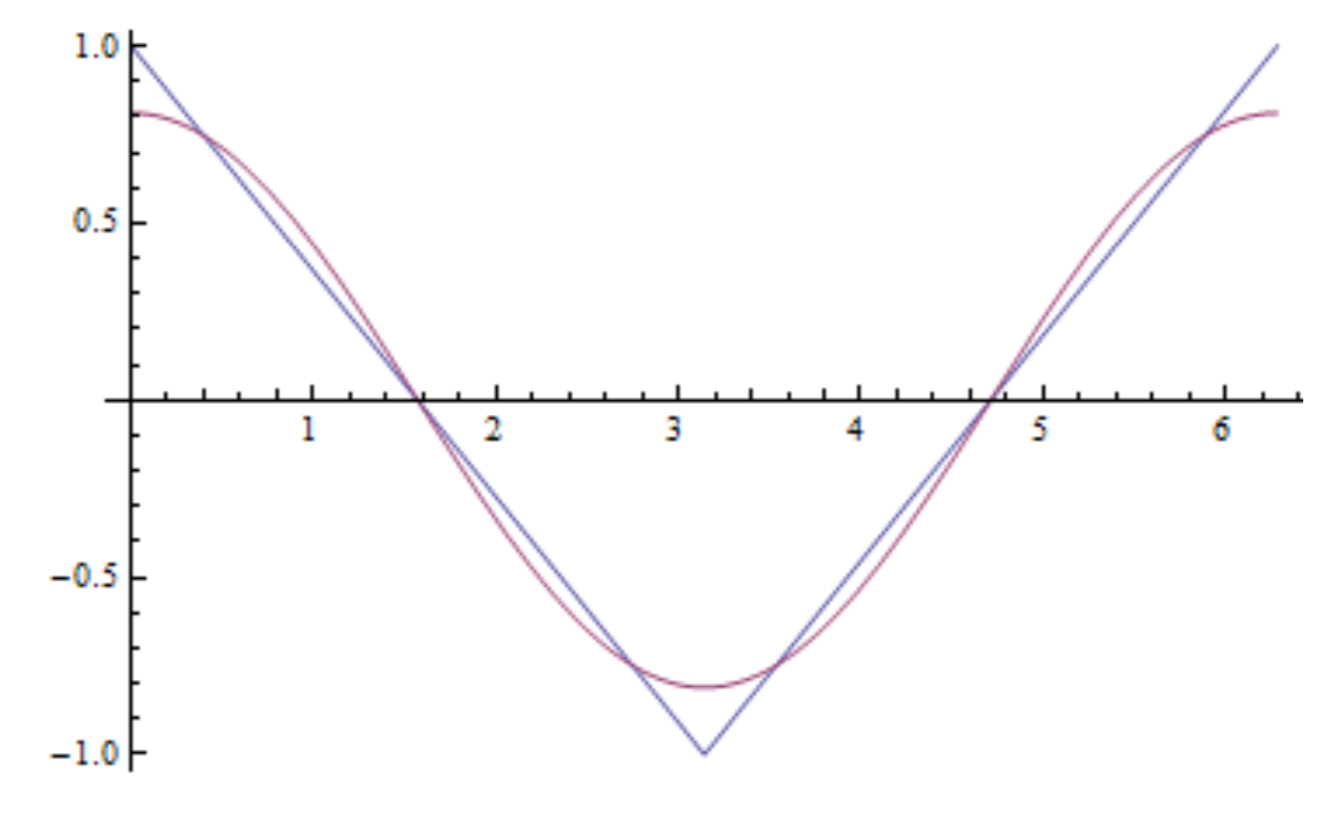
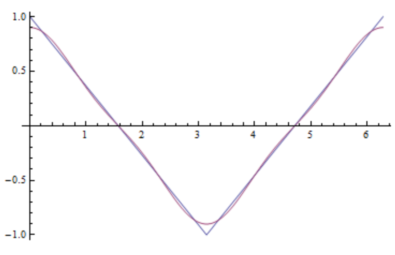
Plot two approximations to your solution, one including the first nonzero term and the other including the first four nonzero terms.
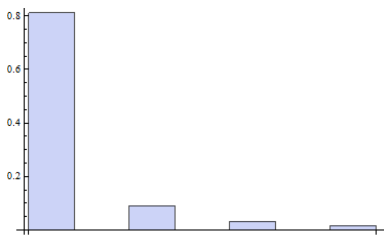
Make a histogram of your coefficients, i.e. find the spectrum.
- Find the Fourier series for a triangle wave (such as the one shown in the figure), which has amplitude \(A\) and period \(T\).
- Fourier Series for the Ground State of a Particle-in-a-Box.
S1 5012S
Treat the ground state of a quantum particle-in-a-box as a periodic function.
- Suppose you want to expand this ground state in a Fourier series. As a first step, set up the integrals for the Fourier coefficients.
The formula for a Fourier series is: \[f(x)=\frac{1}{2}a_0+\sum_{m=1}^{\infty} a_m\cos{\Big(\frac{2\pi m x}{L}\Big)} +\sum_{m=1}^{\infty} b_m\sin{\Big(\frac{2\pi m x}{L}\Big)},\] with formulas for coefficients: \begin{align} a_m&=\frac{2}{L}\int_0^L \cos{\Big(\frac{2\pi m x}{L}}\Big)f(x)\,dx ,\,m=0,1,2,\dots\\ b_m&=\frac{2}{L}\int_0^L\sin{\Big(\frac{2\pi m x}{L}\Big)}f(x)\,dx,\,m= 1,2,3,\dots \end{align}
The formula for the energy eigenstates of the particle-in-a-box is: \[\psi(x)\rightarrow f(x)=\sqrt{\frac{2}{L}}\sin{\Big(\frac{n\pi x}{L}\Big)}; \text{ with }n=1\text{ for ground state},\] and this will be our \(f(x)\) for the Fourier series coefficient calculations.
So the integrals become: \begin{align} a_m&=\frac{2}{L}\int_0^L \cos{\Big(\frac{2\pi m x}{L}}\Big) \sqrt{\frac{2}{L}}\sin{\Big(\frac{\pi x}{L}\Big)}\,dx ,\,m=0,1,2,\dots\\ b_m&=\frac{2}{L}\int_0^L\sin{\Big(\frac{2\pi m x}{L}\Big)} \sqrt{\frac{2}{L}}\sin{\Big(\frac{\pi x}{L}\Big)}\,dx,\,m= 1,2,3,\dots \end{align} Notice that only one half period of the wavefunction fits inside the integration range, so this function is NOT orthogonal to the Fourier sine and cosine basis.
- Now do some sensemaking. Which terms will have the largest coefficients? Explain briefly.
The function we are expanding is entirely positive from \(0\) to \(L\). Since the first coefficient, \(a_0\), is the average value of the function, it is reasonable to expect it to be a large positive contributer to the Fourier series.
The next term, with coefficient \(a_1\), will be a correction to the average. Since \(\cos{(0)}=1\) is positive, it has the opposite shape expected for making the positive average look like the ground state (which is zero at \(x=0\)). Unless the coefficient is negative! \(a_1\) should be large and negative.
A symbolic solution of \[a_m=\frac{2}{L}\int_0^L \cos{\Big(\frac{2\pi m x}{L}}\Big)\sqrt{\frac{2}{L}}\sin{\Big(\frac{\pi x}{L}\Big)}\,dx\] via Wolfram Alpha yields: \[\frac{4\sqrt{\frac{2}{L}}{\cos^2{(\pi m)}}}{\pi-4\pi m^2},\] with \(\cos^2{(\pi m)}=1\) for all integer values of \(m\) making: \[\frac{4\sqrt{\frac{2}{L}}}{\pi-4\pi m^2},\]
which has a term with \(m^2\) in the denominator. Thus, each coefficient gets smaller as the summation continues. Therefore, the first four terms, \[[a_0,a_1,a_2,a_3],\] are the largest coefficients.
- More sensemaking: Are there any coefficients that you know will be zero? Explain briefly.
If you are going to model the particle-in-a-box ground state with a Fourier series, you have to assume that it is periodic. So outside the box, in particular for negative values of \(x\), the function has to be a copy of what it is inside the box. This periodic extension of the ground state is an even function. Therefore its Fourier series must also be even and will only contain cosine terms. All the \(b_m\) coefficients of the sine terms must be zero.
Alternatively, you can argue that since the formula for the \(b_m\) coefficients includes the integral: \[\int_0^L \sin{\Big(\frac{2\pi m x}{L}}\Big)\sin{\Big(\frac{\pi x}{L}\Big)}\,dx.\] The two sine functions are infinite square well functions, which are known to be orthogonal. Sine functions are orthogonal if you integrate over a half period as well as a whole period.
- Now calculate: Using the technology of your choice or by hand, calculate the four largest coefficients. With screen shots or otherwise, show your work.
The integrals can be calculated by using an integral table, a computer algebra system (like Mathematica or Sage), or by hand. (By hand, substitute the exponential forms for sine and cosine. Exponentials are easy to integrate). But whatever the choice, the coefficients are:
\[a_0 =\frac{1}{L}\int_0^L\cancelto{1}{\cos{\Big(\frac{2\pi 0 x}{L}\Big)}}\,\,\,\,\sqrt{\frac{2}{L}}\sin{\Big(\frac{\pi x}{L}\Big)}\,dx=\boxed{\frac{2}{\pi}\sqrt{\frac{2}{L}}}\]
\[a_1 =\frac{2}{L}\int_0^L\cos{\Big(\frac{2\pi (1) x}{L}}\Big) \sqrt{\frac{2}{L}}\sin{\Big(\frac{\pi x}{L}\Big)}\,dx=\boxed{-\frac{4}{3\pi}\sqrt{\frac{2}{L}}}\]
\[a_2 =\frac{2}{L}\int_0^L\cos{\Big(\frac{2\pi (2) x}{L}}\Big) \sqrt{\frac{2}{L}}\sin{\Big(\frac{\pi x}{L}\Big)}\,dx=\boxed{-\frac{4}{15\pi}\sqrt{\frac{2}{L}}}\]
\[a_3 =\frac{2}{L}\int_0^L\cos{\Big(\frac{2\pi (3) x}{L}}\Big) \sqrt{\frac{2}{L}}\sin{\Big(\frac{\pi x}{L}\Big)}\,dx=\boxed{-\frac{4}{35\pi}\sqrt{\frac{2}{L}}}\]
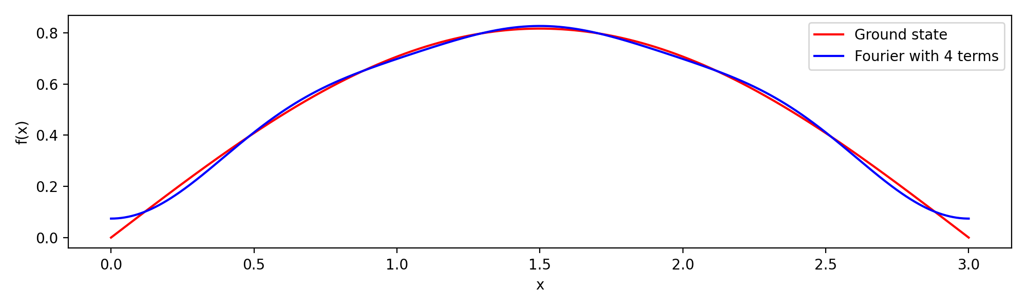
- Using the technology of your choice, plot the ground state and your approximation on the same axes.
The following plot was made using Python, setting \(L=3\).
- Suppose you want to expand this ground state in a Fourier series. As a first step, set up the integrals for the Fourier coefficients.