Quantum Fundamentals: Winter-2026 HW 2 (SOLUTION): Due W1 D5 MathBits
Commutator of Linear Transformations
S1 5413S
Consider the following matrices:
\[A=
\begin{pmatrix}
0&1\\ 1&0\\
\end{pmatrix}\qquad
B=
\begin{pmatrix}
3&1\\ 1&3\\
\end{pmatrix}\qquad
C=
\begin{pmatrix}
1&0\\ 0&-1\\
\end{pmatrix}
\]
Explain what each of the matrices “does” geometrically when thought of as a linear transformation acting on a vector.
Matrix \(A\) reflects vectors over the \(y=x\) line (swaps the components).
Matrix \(C\) reflects vectors over the \(x\)-axis (changes the sign of the \(y\) components).
Matrix \(B\) is a little trickier. I can write \(B\) as:
\begin{align*}
B = 3\begin{pmatrix}1&0\\0&1\end{pmatrix} + 1\begin{pmatrix}0&1\\1&0\end{pmatrix}
\end{align*}
The first term is the identity matrix multiplied by 3, so it just stretches the vector by a factor of 3. The second term is a reflection of the original vector over the line \(y=x\). So the transformation is adding a stretched vector to a reflected vector. The resulting vector is a little longer and a little rotated toward the line \(y=x\). There is not a simple classification for this type of transformation.
Another interpretation is that \(B\) transforms the components of the vector so that the new components are:
\begin{align*}
B\begin{pmatrix}v_x\\v_y\end{pmatrix} = \begin{pmatrix}3v_x+v_y\\v_x+3v_y\end{pmatrix}
\end{align*}
Notice that the components of the new vector are different linear combinations of the original vector components.
The commutator of two matrices \(A\) and \(B\) is defined by \(\left[A,
B\right]\buildrel \rm def \over = AB-BA\). Find the following
commutators: \(\left[A,B\right]\), \(\left[A,C\right]\),
\(\left[B,C\right]\).
Two matrices are said to commute, if their commutator is zero.
It turns out, \(A\) and \(B\) commute:
\begin{align*}
[A,B] &=
\left(\!\!\begin{array}{cc} 0 & 1
\\ 1 & 0 \end{array}\!\!\right)
\left(\!\!\begin{array}{cc} 3 & 1
\\ 1 & 3 \end{array}\!\!\right)
-
\left(\!\!\begin{array}{cc} 3 & 1
\\ 1 & 3 \end{array}\!\!\right)
\left(\!\!\begin{array}{cc} 0 & 1
\\ 1 & 0 \end{array}\!\!\right)\\[6pt]
&=
\left(\!\!\begin{array}{cc} 1 & 3
\\ 3 & 1 \end{array}\!\!\right)
-
\left(\!\!\begin{array}{cc} 1 & 3
\\ 3 & 1 \end{array}\!\!\right)\\[6pt]
&= 0
\end{align*}
The other two commutators are calculated the same way but they do not commute:
\[
[A,C] =
\left(\!\!\begin{array}{cc} 0 & -1
\\ 1 & 0 \end{array}\!\!\right)
-
\left(\!\!\begin{array}{cc} 0 & 1
\\ -1 & 0 \end{array}\!\!\right)
=
\left(\!\!\begin{array}{cc} 0 & -2
\\ 2 & 0 \end{array}\!\!\right),\]
and
\[[B,C] =
\left(\!\!\begin{array}{cc} 0 & -2
\\ 2 & 0 \end{array}\!\!\right).
\]
Thought of as linear transformations, two matrices commute if it
doesn't matter in which order the transformations act. For all pairs
of the matrices \(A\), \(B\), and \(C\), discuss geometrically that the order
of the transformations doesn't matter for the transformations that commute, but that the order does matter when the transformations don't commute.
I'll start with a pair that doesn't commute: transformations \(B\) and \(C\). Since \(C\) reflects over the \(x\)-axis, the mixing of components that \(B\) then performs works very differently, since \(v_x\) has changed the sign. While, when \(B\) is applied first, \(C\) then merely changes the overall sign of one of the components, clearly resulting in a different vector in general. In both these cases the complicated geometrical interpretation of \(B\) forces a more detailed (and partly algebraic) consideration, relying on the component language.
For the pair \(A\) and \(C\), I'll consider a vector in the first quadrant,
and below the \(y=x\) line. If first reflected over \(y=x\), it stays in
the same quadrant, and then reflection over \(x\) sends it to the fourth
quadrant. But if we first reflect over \(x\), it is sent to the fourth
quadrant -- and then reflecting over \(y=x\) must put it in the
second quadrant (since components swap and one is negative,
their signs reverse too). The resulting vectors are thus different.
Since a single case shows that the order of transformations matters, I can stop here. If it didn't matter, this would have to be so for every vector, and so it is sufficient to find one case were it isn't. Showing the commuting property, on the other hand, requires a general case to be proven.
Now for the transformations \(A\) and \(B\). Remember that a vector transformed by \(B\) is the sum of a stretched vector and a vector reflected over the line \(y=x\). Because \(A\) is also a reflection over the line \(y=x\), it doesn't matter which order you do the transformations in. You can either:
stretch the original vector, add it the original vector's reflection over \(y=x\), and then reflect the resultant over \(y=x\), or
reflect the original vector over \(y=x\), stretch the reflected vector, and then add the original vector.
and you get the same result.
Try drawing a few vectors until you convince yourself of the pattern.
Find the normalized vector \(\vert \phi\rangle\) that is orthogonal to it.
Use the property that the scalar product of two vectors that are orthogonal must be zero. We call the vector that we are looking for
\(\left|{\phi}\right\rangle
= \alpha\left|{+}\right\rangle + \beta\left|{-}\right\rangle \).
So we want to take the braket of \(\left|{\psi_{1}^{'}}\right\rangle \) and \(\left|{\phi}\right\rangle \)
Since we are trying to find \(\alpha\) and \(\beta\), it is easier to make \(\left|{\phi_{1}^{'}}\right\rangle \) be the ket so that we do not need to complex conjugate the coefficients that we are trying to determine.
\begin{align*}
0 = \left\langle {\psi}\middle|{\phi}\right\rangle
&= \Big( \frac{1}{\sqrt{3}}
\left\langle {+}\right| + (-i) \frac{\sqrt{2}}{\sqrt{3}} \left\langle {-}\right| \Big)
\Big( \alpha\left|{+}\right\rangle + \beta\left|{-}\right\rangle \Big)\\
&= \frac{\alpha}{\sqrt{3}} - \beta \frac{i\sqrt{2}}{\sqrt{3}}\\
&= 0.
\end{align*}
Then we can choose \(\alpha = \beta \,i\sqrt{2}\), and
\(\alpha = i\sqrt{2}, \ \beta=1\) (for example). There are an infinite number of other choices that we can make that differ from this one by an overall scale. This is because the vector we are finding is orthogonal, but not necessarily normalized. Also, multiplication by an overall phase will not affect the orthogonality.
To normalize, I'll multiply the vector \(\left|{\phi}\right\rangle \) by an overall normalization factor:
\[\left|{\phi}\right\rangle = N \left[ i\sqrt{2} \left|{+}\right\rangle + \left|{-}\right\rangle \right]\]
Find the norm of our choice of vector, I'll take the inner product of the vector with itself and set it equal to 1:
\begin{align*}
1 = \left\langle {\phi}\middle|{\phi}\right\rangle
&=
N^*\begin{pmatrix}
-i\sqrt{2} & 1 \end{pmatrix}
N\begin{pmatrix} i\sqrt{2}
\\ 1 \end{pmatrix}\\
&=|N|^2 (-i\sqrt{2}) \, (i\sqrt{2}) + 1\\ &= 3|N|^2, \\
|N| &= \sqrt{3}.
\end{align*}
The column-vector representation for \(\phi\) is in the
\(\big\{\left|{+}\right\rangle ,\left|{-}\right\rangle \big\}\) basis. Normalized,
\begin{align*}
\left|{\phi}\right\rangle
&=
\frac{1}{\sqrt{3}} \Big( i\sqrt{2} \left|{+}\right\rangle + \left|{-}\right\rangle \Big),
\\ \mathrm{or}\\
\left|{\phi}\right\rangle
&\doteq \frac{1}{\sqrt{3}} \begin{pmatrix} i \sqrt{2}
\\ 1
\end{pmatrix},
\ \mathrm{in~the } \ \Big\{ \left|{+}\right\rangle ,\left|{-}\right\rangle \Big\} \ \mathrm{basis}.
\end{align*}
If I wanted to find \(\phi\) in matrix notation, it would look like:
\begin{align*}
0 = \left\langle {\phi}\middle|{\psi}\right\rangle
&\doteq
\begin{pmatrix} 1/\sqrt{3} & -i\sqrt{2}/\sqrt{3}
\end{pmatrix}
\begin{pmatrix} \alpha
\\ \beta \end{pmatrix}\\
&= \frac{\alpha}{\sqrt{3}} - \beta \frac{i\sqrt{2}}{\sqrt{3}}\\
&= 0
\\ \Rightarrow \; \alpha &= \beta \, i \sqrt{2}.
\end{align*}
Remember that the matrix notation denotes a representation
in some basis.
It should be clear from the context which basis one is working with,
and when it isn't the representation should be stated explicitly. (In the last term
above, the column--vector for \(\left|{\phi}\right\rangle \), is clearly the matrix
representation in the basis \(\big\{\left|{+}\right\rangle ,\left|{-}\right\rangle \big\}\).) Often one
uses the symbol \(\doteq\) to remind ourselves that we are representing a vector in a particular basis.
Graphs of the Complex Conjugate
S1 5413S
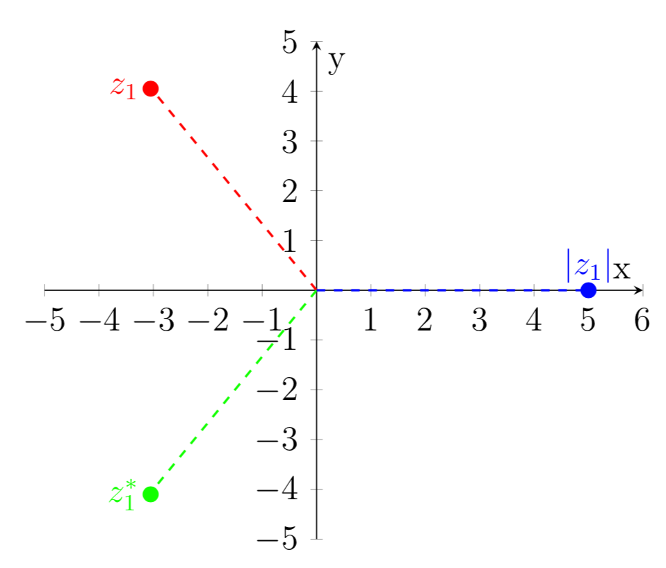
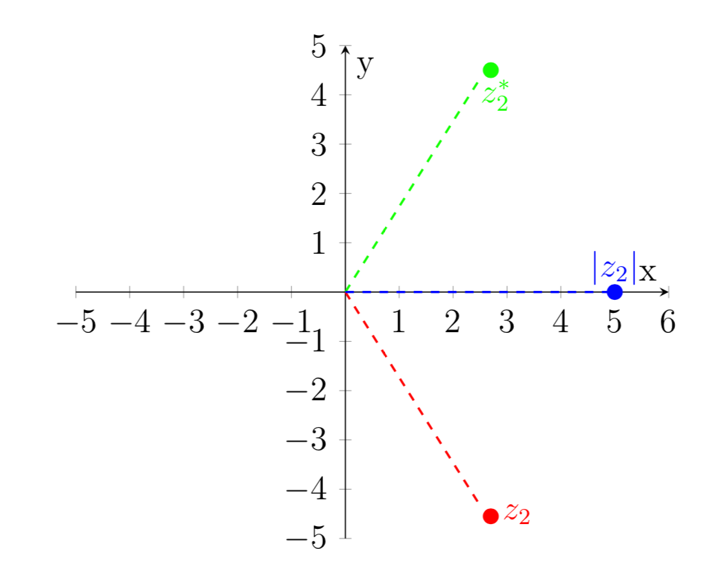
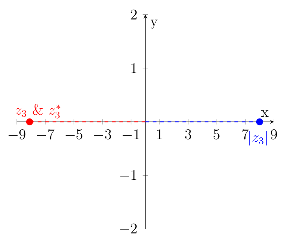
For each of the following complex numbers, determine the complex conjugate, square, and
norm. Then, plot and clearly label each \(z\), \(z^*\), and \(|z|\) on an Argand diagram.
In a few full sentences, explain the geometric meaning of the complex
conjugate and norm.
The complex conjugate reflects the complex number across the real axis while
retaining the distance from the origin. The operation switches the sign of
any \(i\) in the complex number which causes a reflection across the real
axis.
The norm is the distance from the origin to the complex number. The norm
must be a real and positive because it is a length. \(z_1\) and \(z_2\) have
both real and imaginary parts, but their distance from the origin is given
by the norm. For \(z_3\), which is a pure real number, the norm is positive
because it defines the distance the number is from zero.
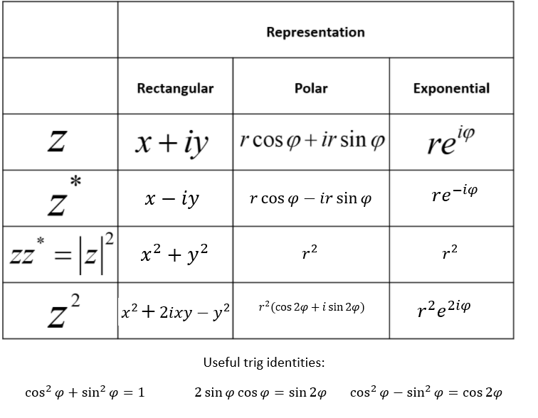
Representations of Complex Numbers--Table
S1 5413S
Fill out the table above that asks you to do several simple complex number calculations in rectangular, polar, and exponential representations.
Note: It is not necessary to simplify using the double-angle formulas in the solution to the polar form of \(z^2\), but it's helpful in the long run if you start learning these rules.