Central Forces: Spring-2026
HW 02 (SOLUTION): Due W1 D5: Math Bits
- Properties of Legendre Polynomials
S1 5532S
-
Use technology such as Mathematica or Maple or Python to find the first 5 Legendre
polynomials. This question is simply asking you to find the command in your preferred computer algebra system and learn the syntax to call the polynomials.
The Mathematica and Maple code for the Legendre polynomial of degree \(\ell\) as a function of \(z\) is: \(LegendreP[\ell,z]\).
In Python, you can use \(legendre(\ell, z)\) from the \(SymPy\) library.
\begin{align*} P_0(z)&=1\\ P_1(z)&=z\\ P_2(z)&=\frac{1}{2}\left(3z^2-1\right)\\ P_3(z)&=\frac{1}{2}\left(5z^3-3z\right)\\ P_4(z)&=\frac{1}{8}\left(35z^4-30z^2+3\right) \end{align*}
-
Use Rodrigues' formula to calculate the first 3 Legendre polynomials. (You
may use computer technology like Mathematica or Maple or Python to help with the
derivatives. This question is asking you to find Rodrigues' formula (Googling it is fine) and learn how to use it to generate the Legendre polynomials.)
Rodrigues' formula is: \[P_{\ell}(z)=\frac{1}{2^{\ell}\ell!} \frac{d^{\ell}}{dz^{\ell}}\left(z^2-1\right)^{\ell}\]
Plugging in for \(\ell=0\)
\begin{align*} P_0(z) &= \frac{1}{2^{0}0!} \left(z^2-1\right)^{0}\\[6pt] &= \frac{1}{(1)(1)} (1)\\[6pt] P_0(z) &= 1 \end{align*}
For \(\ell=1\)
\begin{align*} P_1(z) &= \frac{1}{2^{1}1!} \frac{d}{dz} \left(z^2-1\right)\\[6pt] &= \frac{1}{2} 2z\\[6pt] P_1(z) &= z \end{align*}
For \(\ell = 2\) \begin{align*} P_2(z) &= \frac{1}{2^{2}2!} \frac{d^2}{dz^2} \left(z^2-1\right)^2\\[6pt] &= \frac{1}{(4)(2)} \frac{d}{dz}\Big[2(z^2-1)(2z)\Big]\\[6pt] P_2(z) &= \frac{1}{2}(3z^2-1) \end{align*}
-
Use technology such as Mathematica or Maple or Python to find the first 5 Legendre
polynomials. This question is simply asking you to find the command in your preferred computer algebra system and learn the syntax to call the polynomials.
- Legendre Polynomial Series for the Sine Function
S1 5532S
Use your favorite technology tool (e.g. Maple, Mathematica, Matlab, Python, pencil) to generate the Legendre polynomial expansion to the function \(f(z)=\sin(\pi z)\). How many terms do you need to include in a partial sum to get a “good” approximation to \(f(z)\) for \(-1<z<1\)? What do you mean by a “good” approximation? How about the interval \(-2<z<2\)? How good is your approximation? Discuss your answers. Answer the same set of questions for the function \(g(z)=\sin(3\pi z)\)
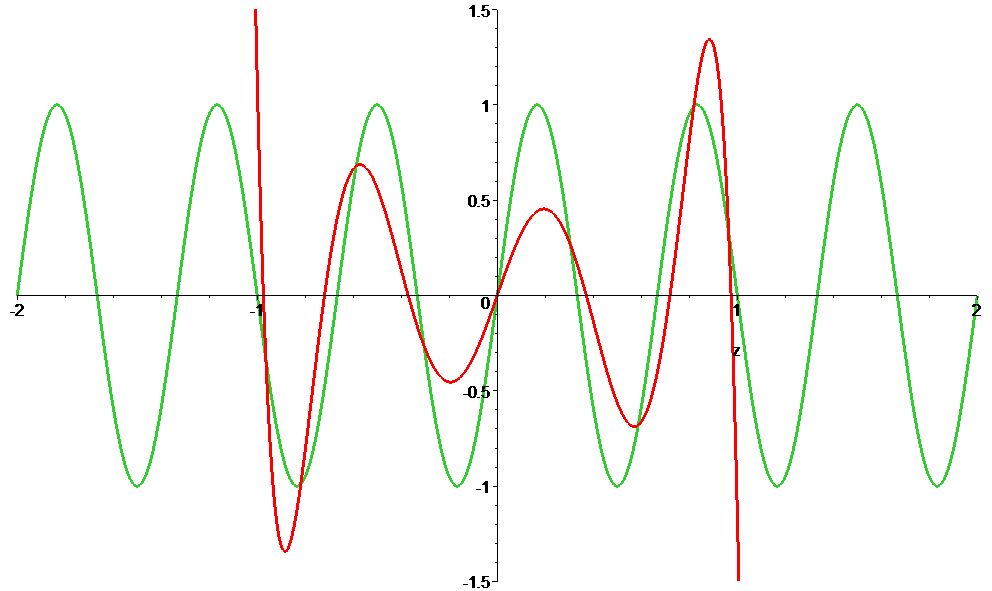
The function \(\sin(\pi\, z)\) is an odd function, therefore we only expect to get contributions from Legendre polynomials with odd values of \(\ell\). For \(\ell=1\), we will get a straight line approximation to the sine function, surely not good enough. For \(\ell=3\) we see that we are already getting the right number of peaks for the range \(-1<z<1\), but the peaks are shifted and not quite the right shape. For \(\ell=5\), we are already getting a reasonably good fit, depending on our needs. As always, we need to say “a good fit compared to what?”. Notice, however, that outside the range of \(-1<z<1\), the fit gets worse and worse as we add more terms. See for example, this graph for \(\ell=19\). This behavior is expected. Series of orthogonal polynomials each have a specified region of convergence. For Legendre polynomials, the region of convergence is \(-1<z<1\).
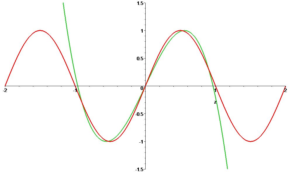
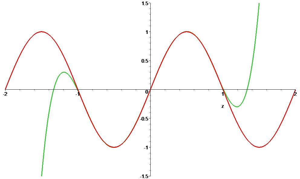
The Legendre Series approximation for the function \(\sin(\pi z)\) terminating at \(\ell=3\) (left) and \(\ell=5\) (right). 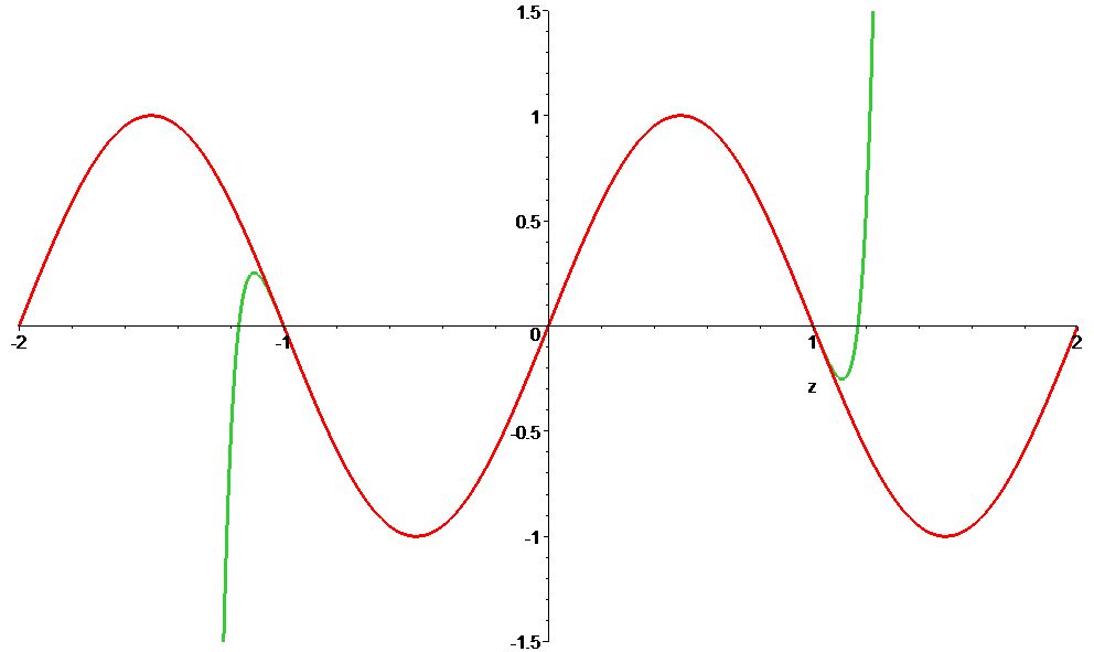
The Legendre Series approximation for the function \(\sin(\pi z)\) terminating at \(\ell=19\). For the function \(\sin(3\pi\, z)\), terminating the series at \(\ell=3\) is a terrible fit. It doesn't even have enough terms to fit the correct number of peaks. Remember that the Legendre polynomials are polynomials, so terminating the series at \(\ell=3\) gives you only two peaks. For \(\ell=7\), we are at least getting the correct number of peaks. And for \(\ell=13\), we are finally getting the same kind of fit that we got in the previous example for \(\ell=5\).
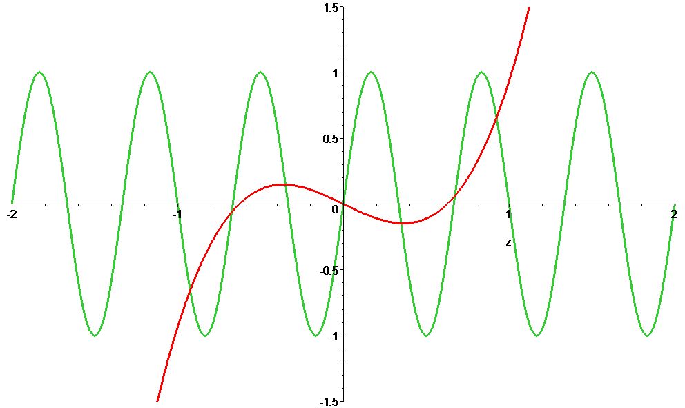
The Legendre Series approximation for the function \(\sin(3\pi z)\) terminating at \(\ell=3\) (left) and \(\ell=7\) (right). 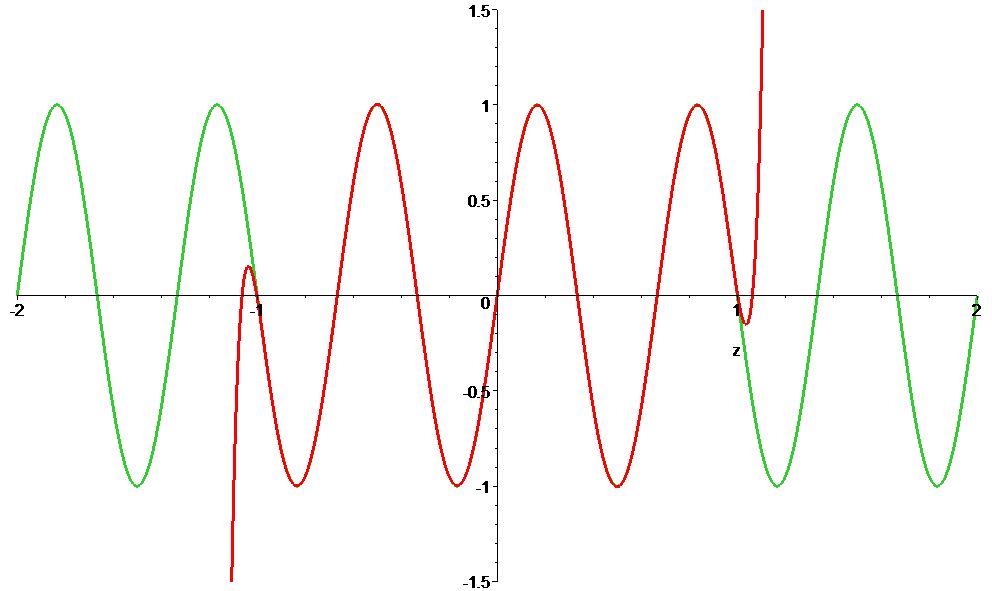
The Legendre Series approximation for the function \(\sin(3\pi z)\) terminating at \(\ell=13\). - Laplace's Equation in Polar Coordinates
S1 5532S
- Write down Laplace's equation in two dimensions in polar coordinates.
\begin{align*} \nabla^2 f &= 0 \\ \vec{\nabla}\cdot\vec{\nabla} f&=0\\ \frac{\partial^2 f}{\partial r^2}+\frac{1}{r}\frac{\partial f}{\partial r}+\frac{1}{r^2}\frac{\partial ^2 f}{\partial \phi^2} &= 0 \end{align*}
- Use the separation of variables procedure to separate this partial differential equation into two ordinary differential equations.
To separate the equation, first write the solution as a product of functions, one for each variable. \begin{align*} f(r,\phi)=R(r)\Phi(\phi) \end{align*}
Plug this ansatz into the differential equation:
\begin{align*} \frac{\partial^2 R}{\partial r^2}\Phi+\frac{1}{r}\frac{\partial R}{\partial r}\Phi+\frac{1}{r^2}R\frac{\partial ^2 \Phi}{\partial \phi^2}=0 \end{align*} Divide by \(f\) in the form of \(f=R\Phi\): \begin{align*} \frac{1}{R}\frac{\partial^2 R}{\partial r^2}+\frac{1}{r}\frac{1}{R}\frac{\partial R}{\partial r}+\frac{1}{r^2}\frac{1}{\Phi}\frac{\partial ^2 \Phi}{\partial \phi^2}=0 \end{align*} And then multiply through by \(r^2\) and put all of the \(r\) dependence on one side of the equation and all the \(\phi\) dependence on the other side of the equation. \begin{align*} r^2\,\frac{1}{R}\frac{\partial^2 R}{\partial r^2}+r\,\frac{1}{R}\frac{\partial R}{\partial r}=-\frac{1}{\Phi}\frac{\partial ^2 \Phi}{\partial \phi^2}\\ \end{align*} Utter the magic words: "Since the left-hand side of the equation could depend on \(r\), but the right-hand side does not, if we change \(r\) by a little bit, the right-hand side of the equation remains constant. Therefore, the particular combination of \(r\) dependences on the left-hand side of the equation must also be constant. Ditto for the \(\phi\) dependence with the role of left- and right-hand sides of the equation reversed. We can therefore set both sides of the equation equal to the SAME constant \(D\)." \begin{align*} D&=r^2\,\frac{1}{R}\frac{\partial^2 R}{\partial r^2}+r\,\frac{1}{R}\frac{\partial R}{\partial r}\\ D&=-\frac{1}{\Phi}\frac{\partial ^2 \Phi}{\partial \phi^2}\\ &\Rightarrow\\ DR&=r^2\,\frac{\partial^2 R}{\partial r^2}+r\,\frac{\partial R}{\partial r}\\ D\Phi&=-\frac{\partial ^2 \Phi}{\partial \phi^2}\\ \end{align*}
- Write down a complete set of eigenstates of the \(\phi\) equation. Justify your answer. You do not NEED to calculate anything here, but if you quote some answer that you already know, say how/where you know the answer. DO NOT TRY TO SOLVE THE \(r\) EQUATION!
This is a second order differential equation, so we expect two solutions: \begin{align*} \Phi(\phi)&=A\cos( \sqrt{D}\phi)+B\sin ( \sqrt{D}\phi)\\ \text{or}&\\ \Phi(\phi)&=C_1\exp (i\sqrt{D}\phi)+C_2\exp (-i\sqrt{D}\phi)\\ \end{align*} To make these solutions satisfy periodic boundary conditions \(\Phi(\phi+2\pi)=\Phi(\phi)\), we must have \(\sqrt{D}=\left\{0, \pm 1, \pm 2, \pm 3, \dots\right\}\).
- Write down Laplace's equation in two dimensions in polar coordinates.
- Chain rule for changing 1 independent variable
S1 5532S
- Use the chain rule to show that \(\frac{d}{dt} = v \frac{d}{dx}\).
\begin{align*} \frac{d}{dt} &= \frac{dx}{dt}\frac{d}{dx} \\ &= v \; \frac{d}{dx} \end{align*}
- A point particle moving along the \(x\)-axis with an initial speed \(v_0 \neq 0 \) is subject to a linear drag force as described by the equation: \(\frac{dv}{dt} = -\frac{b}{m}v\), where \(b\) and \(m\) are constants. Find \(v(x)\).
\begin{align*} \frac{dv}{dt} &= -\frac{b}{m}v\\ \cancel{v}\frac{dv}{dx} &= -\frac{b}{m}\cancel{v} \\ dv &= -\frac{b}{m} dx\\ \int_{v_0}^{v}dv' &= -\int_{x_0}^{x}\frac{b}{m} dx'\\ v(x) &= v_0 - \frac{b}{m}(x-x_0) \end{align*}
- Use the chain rule to represent the operator \(\frac{d}{d\theta}\) in terms of the cartesian coordinate \(z\) on the unit sphere.
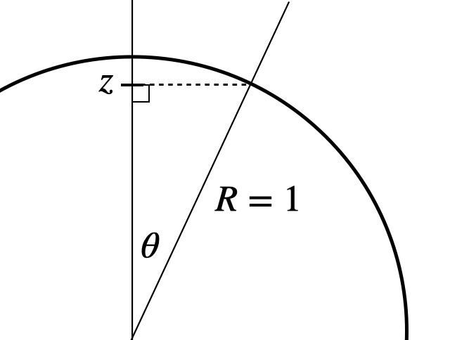
- Hint 1: Draw a picture and think triangles.
- Hint 2: Be sure to substitute all the \(\theta\)'s for z's.
First, when I draw my picture, I see that \(z=\cos\theta\).
Next, I'll think about the chain rule:
\begin{align*} \frac{d}{d\theta} = \frac{dz}{d\theta}\frac{d}{dz} \end{align*}
where I have aligned the differentials so they cancel appropriately.
To find \(\frac{dz}{d\theta}\), from my picture:
\begin{align*} z &= \cos\theta \\ \frac{dz}{d\theta} &= -\sin\theta \end{align*}
Plugging in, I get
\begin{align*} \frac{d}{d\theta} = -\sin\theta\;\frac{d}{dz} \end{align*}
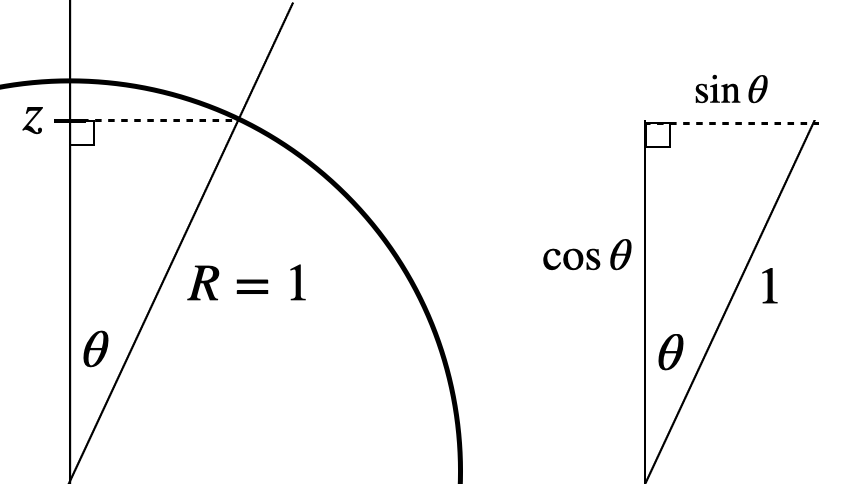
But I'm not done, because I still have a \(\theta\) on the right-hand-side. Going back to my picture and using Pythagorean Theorem and triangle trig, I see that:
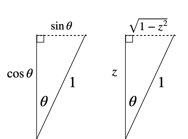
\begin{align*} \sin\theta = \sqrt{1-z^2} \end{align*}
Therefore,
\begin{align*} \frac{d}{d\theta} = -\sqrt{1-z^2}\;\frac{d}{dz} \end{align*}
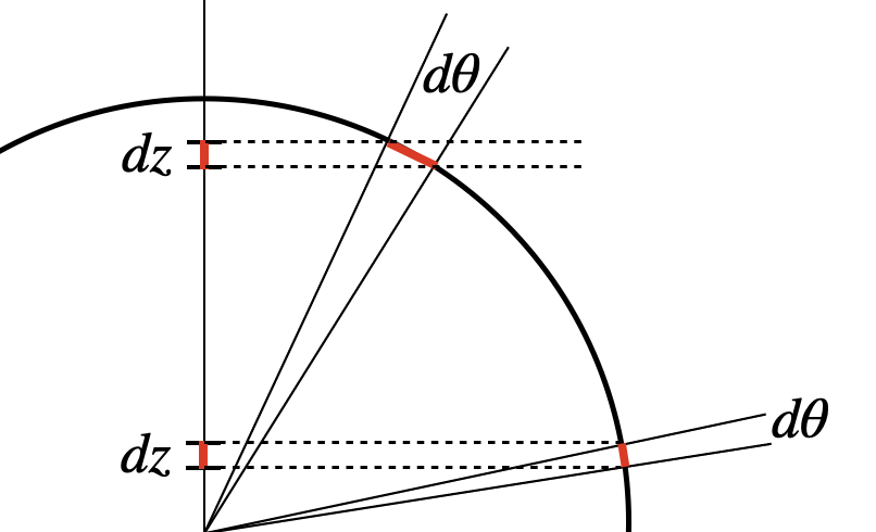
To make geometric sense of this, I'll rewrite it as:
\begin{align*} {d\theta} = -\frac{dz}{\sqrt{1-z^2}} \end{align*}
To me, this makes sense because if \(z\) is near 0, then changes in \(z\) and \(\theta\) are about the same (remember, there is an \(R = 1\) for the unit sphere hidden in this expression). This matches my picture.
However, as I get near the poles of the sphere, \(z^2\) approaches 1, the denominator on the right-hand-side gets smaller, indicating that a small change in \(z\) corresponds to the relatively larger change in \(\theta\). Again, this matches my picture.
- Use the chain rule to show that \(\frac{d}{dt} = v \frac{d}{dx}\).