Periodic Systems: Spring-2026
HW 4 (SOLUTION): Due Day 10
- Particle in a Box Solve Schrodinger
S1 5495S
Consider a quantum particle with mass \(m\) in a 1-D box where the potential is:
\begin{align*}
V = \begin{cases}
\infty & x< 0\\
0 & 0 \leq x \leq L \\
\infty & L<x
\end{cases}
\end{align*}
What is the Hamiltonian for this system?
The Hamiltonian is the sum of the kinetic and potential energies:
\[\hat{H} = \hat{T} + \hat{V}\]
Inside the well, the Hamiltonian is:
\begin{align*} \hat{H} &= \hat{T} + \cancelto{0}{\hat{V}}\\ &= -\frac{\hbar^2}{2m}\frac{\partial^2}{\partial x^2} \end{align*}
Outside the well, the Hamiltonian is infinite and therefore not useful.
Use a separation of variables procedure to solve the Schrödinger Equation for this system and find the general solution \(\Phi(x,t)\). (You saw the solution in Ph425 but now I want you to solve it yourself.)
I'll make the ansatz that the \(x\) and \(t\) dependence is separable, \(\Phi(x,t) = \phi(x)\tau(t)\), and plug this guess into the Schrödinger Equation:
\[-\frac{\hbar^2}{2m}\frac{\partial^2 \phi(x)\tau(t)}{\partial x^2} = i\hbar\frac{\partial \phi(x)\tau(t)}{\partial t}\]
Then I pull out of each partial derivative any quantity that is held constant with respect to that variable.
\[-\tau(t)\frac{\hbar^2}{2m}\frac{\partial^2 \phi(x)}{\partial x^2} = i\hbar\phi(x)\frac{\partial \tau(t)}{\partial t}\]
Then I divide both sides by \(\phi(x,t) = \phi(x)\tau(t)\) in order to separate the variables: all \(x\) on the left and all \(t\) on the right.
\[-\frac{\hbar^2}{2m}\frac{1}{\phi(x)}\frac{\partial^2 \phi(x)}{\partial x^2} = i\hbar\frac{1}{\tau(t)}\frac{\partial \tau(t)}{\partial t}\]
This equation now tells me that a function only of \(x\) is identically equal to a function only of \(t\) for all values of both \(x\) and \(t\). This can only be true if each side of the above equation is equal to the same constant. For real physical reasons, I choose to name that constant \(E\) (for energy). I then first solve the resulting spatial equation:
\[-\frac{\hbar^2}{2m}\frac{1}{\phi(x)}\frac{\partial^2 \phi(x)}{\partial x^2} = E\]
\[\frac{\partial^2 \phi(x)}{\partial x^2} = -\frac{2mE}{\hbar^2}\phi(x)\]
This is the energy eigenvalue equation and I happen to already know the solution. I will guess to start out with that \(E\) is positive (this is reasonable since the energy is only kinetic energy). I also introduce a temporary shorthand variable \(k = \sqrt{\frac{2mE}{\hbar^2}}\) for ease of writing.
\[\phi(x) = A\cos(kx) + B\sin(kx)\]
Now I'll apply the boundary conditions.
- First, \(\phi(0,t)=0\) implies that \(\phi(0)=0\), so \(\phi(0) = A + 0 = 0\) and thus \(A = 0\).
- Second, \(\phi(L,t)=0\) implies that \(\phi(L)=0\), so \(\phi(0) = B\sin(kL) = 0\). Since choosing \(B=0\) gives a physically uninteresting solution of 0 everywhere, this equation does not give me a condition on \(B\) but instead on \(k\)! That condition is that I must choose a value of \(k\) that makes the sine vanish, which is \(kL = n\pi\), or \(k = n\pi/L\).
Third, I need to make sure my solution is normalized:
\begin{align*} 1 &= \int_0^L |\phi(x)|^2 dx\\ &= \int_0^L |B|^2\sin^2(\frac{n\pi x}{L})dx\\ &= |B|^2\frac{L}{2} \end{align*}
Therefore, \(B=\sqrt{\frac{2}{L}}\). Notice that it is the same for all values of \(n\)!
The solution for the \(x\) equation is therefore:
\[\phi_n(x) = \sqrt{\frac{2}{L}}\sin(\frac{n\pi x}{L})\]
Now we turn back to the \(t\) equation. Note that my knowledge of \(k\) gives me a new expression for \(E\), which is also now dependent on \(n\): \(E_n = \frac{n^2\pi^2\hbar^2}{2mL^2}\). Since this is a lot, I will continue to use the shorthand of \(E_n\), and will also add this label to the function \(\tau(t)\).
\[i\hbar\frac{1}{\tau_n(t)}\frac{\partial \tau_n(t)}{\partial t} = E_n\]
\[\frac{\partial \tau_n(t)}{\partial t} = -i\frac{E_n}{\hbar}\tau_n(t)\]
Once again, the solution of this equation is very familiar--an exponential! Note that this looks like the equation for a real exponential, but the imaginary coefficient in the equation itself turns it into an imaginary exponential. Also note that sines and cosines may prove less useful here, so I leave the result in terms of \(i\).
\[\tau_n(t) = Ce^{-iE_n t/\hbar}\]
This solution should look very familiar, as it is always the time-dependent part of solving the Schrodinger equation as long as you have Hamiltonians (i.e., systems) that are independent of time. I don't have any initial conditions yet, so this is the solution to the \(t\) side of the equation. Now, however, I have to put it back together with the \(x\) solution to get:
\[\phi_n(x,t) = \phi_n(x)\tau_n(t) = \sqrt{\frac{2}{L}}\sin(\frac{n\pi x}{L}) Ce^{-iE_n t/\hbar}\]
The general solution of the Schrödinger Equation is a linear combination of terms with different \(n\)'s:
\[\phi(x,t) = \sum_{n=1}^{\infty}c_n\sqrt{\frac{2}{L}}\sin(\frac{n\pi x}{L}) e^{-in^2\pi^2\hbar t/2mL^2}\]
where I have absorbed the coefficient \(C\) into the expansion coefficient \(c_n\) and plugged in the energy eigenvalues.
- Particle in a Box Review
S1 5495S
As a review of the infinite square well system, consider a quantum particle with mass \(m\) is a 1-D box from \(0\leq x \leq L\). The initial state of the particle is:
\[\psi(x,0) = \sqrt{\frac{2}{3L}}\sin\left(\frac{2\pi x}{L}\right) + \frac{2i}{\sqrt{3L}}\sin\left(\frac{3\pi x}{L}\right)\]
Write down the energy eigenvalues and eigenstates for this system. (You don't have to re-solve for them in this problem.)
The energy eigenvalues are:
\[E_n = \frac{n^2\pi^2\hbar^2}{2mL^2}\]
The energy eigenstates are:
\[|E_n\rangle \doteq \phi_n(x) = \sqrt{\frac{2}{L}} \;\sin \Big( \frac{n\pi x}{L}\Big)\]
If you measured the energy of the system at \(t=0\), what is the probability you would measure the value \(E = 9\pi^2\hbar^2/2mL^2\)?
I recognize that this initial state is a linear combination of energy eigenstates:
\begin{align*} \psi(x,0) &= \frac{1}{\sqrt{3}}\Big[\sqrt{\frac{2}{L}}\sin(\frac{2\pi x}{L})\Big] + \sqrt{\frac{2}{3}} \Big[ \sqrt{\frac{2}{L}}\sin(\frac{3\pi x}{L})\Big]\\ \left|{\psi}\right\rangle &= \frac{1}{\sqrt{3}}\;\left|{E_2}\right\rangle + \sqrt{\frac{2}{3}}\; \left|{E_3}\right\rangle \\ \end{align*}
where the first term corresponds to \(E_2 = \frac{4\pi^2\hbar^2}{2mL^2}\) and the second term corresponds to \(E_3 = \frac{9\pi^2\hbar^2}{2mL^2}\).
The probabilities are the norm square of the projection of the state onto the corresponding basis element:
\begin{align*} \mathcal{P}(E_2) &= \left| \left\langle {E_2}\middle|{\psi}\right\rangle \right|^2 \\ &= \left| \frac{1}{\sqrt{3}} \right|^2 \\ &= \frac{1}{3} \\[12pt] \mathcal{P}(E_3) &= \left| \left\langle {E_3}\middle|{\psi}\right\rangle \right|^2 \\ &= \left|i \sqrt{\frac{2}{3}} \right|^2 \\ &= \frac{2}{3}\\ \end{align*}
What is the expectation value of the energy at \(t=0\)
Conceptually, the expectation value is the average of the values that can be measured:
\begin{align*} \langle E \rangle &= \sum_n \mathcal{P}_nE_n \\[6pt] &= \frac{1}{3}\frac{4\pi^2\hbar^2}{2mL^2} + \frac{2}{3}\frac{9\pi^2\hbar^2}{2mL^2} \\[6pt] &= \frac{\pi^2\hbar^2}{2mL^2} \Big[\frac{4}{3} + \frac{18}{3} \Big] \\[6pt] &= \frac{11\pi^2\hbar^2}{3mL^2} \end{align*}
This can also be found through integration:
\begin{align*} \langle E \rangle &= \int_0^L \psi^*(x)\, \hat{H} \, \psi(x)\; dx \\[6pt] &= \int_0^L \psi^*(x)\, \Bigg(-\frac{\hbar^2}{2m}\frac{\partial^2}{\partial x^2} \, \psi(x)\Bigg) \; dx \\[12pt] &= \int_0^L \Big[\sqrt{\frac{2}{3L}}\sin(\frac{2\pi x}{L}) + \frac{2i}{\sqrt{3L}}\sin(\frac{3\pi x}{L})\Big] \\&\Bigg(-\frac{\hbar^2}{2m}\frac{\partial^2}{\partial x^2} \, \Big[\sqrt{\frac{2}{3L}}\sin(\frac{2\pi x}{L}) + \frac{2i}{\sqrt{3L}}\sin(\frac{3\pi x}{L})\Big]\Bigg) \; dx \\[12pt] &= -\frac{\hbar^2}{2m}\int_0^L \Big[\sqrt{\frac{2}{3L}}\sin(\frac{2\pi x}{L}) + \frac{2i}{\sqrt{3L}}\sin(\frac{3\pi x}{L})\Big] \\&\Big[\sqrt{\frac{2}{3L}}\Big(-\frac{4\pi^2}{L^2}\Big)\sin(\frac{2\pi x}{L}) + \frac{2i}{\sqrt{3L}}\Big(-\frac{9\pi^2}{L^2}\Big)\sin(\frac{3\pi x}{L})\Big]\Bigg) \; dx \\[12pt] &= \frac{11\pi^2\hbar^2}{3mL^2} \end{align*}
What is the uncertainty of the energy at \(t=0\)
The uncertainty is the standard deviation of the distribution of energies.
\begin{align*} \Delta E &= \sqrt{\langle \hat{H}^2 \rangle - \langle \hat{H} \rangle^2} \\[12pt] \langle H \rangle^2 &= \Big(\frac{11\pi^2\hbar^2}{3mL^2}\Big)^2 = \Big(\frac{\pi^2\hbar^2}{mL^2}\Big)^2 \Big(\frac{11}{3}\Big)^2 \\[6pt] \langle \hat{H^2} \rangle &= \sum_n \mathcal{P}_nE_n^2 \\[12pt] &= \frac{1}{3}\Big(\frac{4\pi^2\hbar^2}{2mL^2}\Big)^2 + \frac{2}{3}\Big(\frac{9\pi^2\hbar^2}{2mL^2}\Big)^2 \\[12pt] &= \Big(\frac{\pi^2\hbar^2}{mL^2}\Big)^2 \Big( \frac{4^2}{3(2^2)} + \frac{2(9^2)}{3(2^2)} \Big) \\[12pt] &= \Big(\frac{\pi^2\hbar^2}{mL^2}\Big)^2 \Big( \frac{(4^2+2(9^2))}{3(2^2)} \Big) \\[12pt] \Delta E &= \sqrt{\Big(\frac{\pi^2\hbar^2}{mL^2}\Big)^2 \Big( \frac{(4^2+2(9^2))}{3(2^2)} \Big) - \Big(\frac{\pi^2\hbar^2}{mL^2}\Big)^2 \Big(\frac{11}{3}\Big)^2} \\[12pt] &= \frac{\pi^2\hbar^2}{mL^2}\sqrt{\Big( \frac{3(4^2+2(9^2))}{(3^2)(2^2)} \Big) - \Big(\frac{11^2(2^2)}{(3^2)(2^2)}\Big)} \\[12pt] &= \frac{\pi^2\hbar^2}{mL^2}\sqrt{ \frac{25}{18} } \\[12pt] \end{align*}
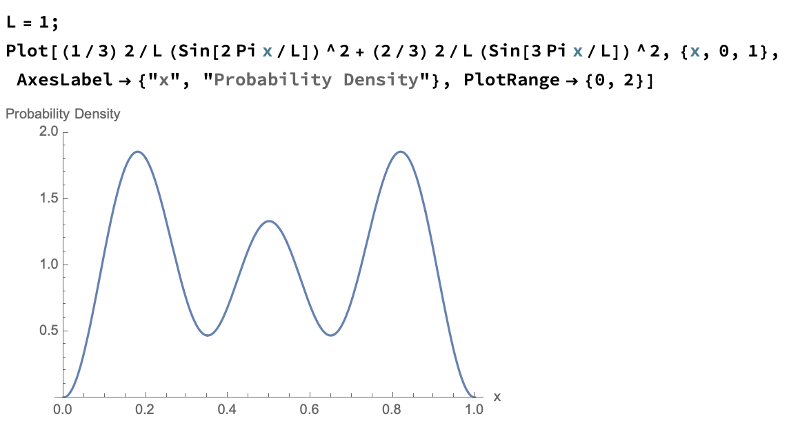
Plot the probability density of the system.
The probability density is the norm square of the wavefunction.
\begin{align*} |\psi(x)|^2 &= \left|\sqrt{\frac{2}{3L}}\sin(\frac{2\pi x}{L}) + \frac{2i}{\sqrt{3L}}\sin(\frac{3\pi x}{L}) \right|^2 \\ &= \left|\sqrt{\frac{2}{3L}}\sin(\frac{2\pi x}{L})\right|^2 + \left|\frac{2}{\sqrt{3L}}\sin(\frac{3\pi x}{L})\right|^2 \end{align*}
If instead you measured the position of the system at \(t=0\), what is the probability you would find the particle between \(x=L/4\) and \(x=L/2\)?
To calculate this, I integrate the probability density over the region:
\begin{align*} \mathcal{P}(L/4<x<L/2) &= \int_{L/4}^{L/2} |\psi(x)|^2 dx \\[12pt] &= \int_{L/4}^{L/2} \Bigg|\sqrt{\frac{2}{3L}}\sin(\frac{2\pi x}{L}) + \frac{2i}{\sqrt{3L}}\sin(\frac{3\pi x}{L})\Bigg|^2 dx \\[12pt] &= \int_{L/4}^{L/2} \Bigg|\sqrt{\frac{2}{3L}}\sin(\frac{2\pi x}{L})\Bigg|^2 dx + \\ & \quad\int_{L/4}^{L/2}\Bigg|\frac{2}{\sqrt{3L}}\sin(\frac{3\pi x}{L})\Bigg|^2 dx \\[12pt] &= \frac{1}{12} + \frac{1}{6} - \frac{1}{9\pi} \\ &= \frac{1}{4} - \frac{1}{9\pi} \\[12pt] &\approx 0.21 \end{align*}
I'm comforted that this value is between 0 and 1, which makes sense for a probability. It also looks like it's about 1/5, which matches the graph of the probability density.
What will be the state of this particle at a later time \(t\)?
I recognize that this initial state is a linear combination of energy eigenstates:
\begin{align*} \psi(x,0) &= \frac{1}{\sqrt{3}}\Big(\sqrt{\frac{2}{L}}\sin(\frac{2\pi x}{L})\Big) + \sqrt{\frac{2}{3}} \Big( \sqrt{\frac{2}{L}}\sin(\frac{3\pi x}{L})\Big)\\ \end{align*}
where the first term corresponds to \(E_2 = \frac{4\pi^2\hbar^2}{2mL^2}\) and the second term corresponds to \(E_3 = \frac{9\pi^2\hbar^2}{2mL^2}\)
Plugging this information into the general solution, I get:
\begin{align*} \psi(x,t) =& \sum_{n=1}^{\infty}c_n\sqrt{\frac{2}{L}}\sin(\frac{n\pi x}{L}) e^{-iE_n t/\hbar}\\ =& c_2\sqrt{\frac{2}{L}}\sin(\frac{2\pi x}{L}) e^{-iE_2 t/\hbar}+c_3\sqrt{\frac{2}{L}}\sin(\frac{3\pi x}{L}) e^{-iE_3 t/\hbar}\\ =&\frac{1}{\sqrt{3}}\sqrt{\frac{2}{L}}\sin(\frac{2\pi x}{L}) e^{-i4\pi^2 \hbar t/2mL^2}\\ &+i\sqrt{\frac{2}{3}}\sqrt{\frac{2}{L}}\sin(\frac{3\pi x}{L}) e^{-i9\pi^2\hbar t/2mL^2}\\ \end{align*}