Central Forces: Spring-2026
HW 07 (SOLUTION): Due W4 D3
- Ring Function
S1 5542S
Consider the normalized wavefunction \(\Phi\left(\phi\right)\) for a
quantum mechanical particle of mass \(\mu\) constrained to move on a
circle of radius \(r_0\), given by:
\begin{equation}
\Phi\left(\phi\right)= \frac{N}{2+\cos(3\phi)}
\end{equation}
where \(N\) is the normalization constant.
Find \(N\).
See the attached Mathematica notebook for the value of the integrals in this problem and for the code for the plots.
To find \(N\), normalize the wave function. \begin{align} \int_{0}^{2\pi} \left|\Phi\right|^2\,r_0\,d\phi &= 1\\ |N|^2\,r_0 \int_{0}^{2\pi} \frac{1}{(2+\cos{3\phi})^2}\,d\phi &= 1\\ |N|^2\,r_0 \left(\frac{4\sqrt{3}\pi}{9}\right) &= 1\label{norm}\\ N &= \frac{3^{3/4}}{2\sqrt{\pi r_0}} \end{align} where in Eqn. (\ref{norm}) we have evaluated the integral using Mathematica.
-
Plot this wave function.
The unnormalized wavefunction is \(\frac{1}{2+\cos{3\phi}}\)
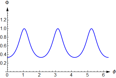
A plot of the wave function \(\Phi(\phi)\). - Plot the probability density.
The probability density is \(\left\vert \frac{1}{2+3\cos\phi}\right\vert^2\).
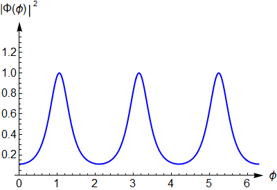
A plot of the probability density \(\vert\Phi(\phi)\vert^2\). - Find the probability that if you measured \(L_z\) you would get \(3\hbar\).
\begin{align} \mathcal{P}(L_z=3\hbar)&=\left\vert\left\langle {3}\middle|{\Phi}\right\rangle \right\vert^2\\ &=\left\vert\int_0^{2\pi} \left(\frac{1}{\sqrt{2\pi r_0}}e^{-3i\phi}\right) \left(\frac{N}{2+\cos(3\phi)}\right)\, r_0\, d\phi \right\vert^2\\ &=\left\vert\int_0^{2\pi} \left(\frac{1}{\sqrt{2\pi r_0}}(\cos{3\phi}-i\sin{3\phi})\right) \left(\frac{N}{2+\cos(3\phi)}\right)\, r_0\, d\phi \right\vert^2\\ &=\frac{\vert N\vert^2\, r_0}{2\pi}\left\vert\int_0^{2\pi} \left(\left(\frac{\cos{3\phi}}{2+\cos(3\phi)}\right) -\left(\frac{\sin{3\phi}}{2+\cos(3\phi)}\right)\right)\, d\phi \right\vert^2\label{Lz}\\ &=\frac{\vert N\vert^2\, r_0}{2\pi} \left\vert\left(2-\frac{4}{\sqrt{3}}\right)\pi+0\right\vert^2\\ &=\frac{\sqrt{3}}{2}\left(\sqrt{3}-2\right)^2 \end{align} where in Eqn. (\ref{Lz}) we have evaluated the integral using Mathematica. See the attached notebook.
-
What is the expectation value of \(L_z\) in this state?
In the position representation, \(L_z=-i\hbar \frac{d}{d\phi}\) is a differential operator. Make sure to sandwich it between the "bra" and "ket" and only let it operate on the "ket." \begin{align} \langle L_z \rangle &= \int_{0}^{2\pi}\Phi^*\hat{L_z}\Phi\,r_0\,d\phi\\ &= \int_{0}^{2\pi} \frac{N}{2+\cos{3\phi}} \; \left(-i\hbar \frac{d}{d \phi}\right) \frac{N}{2+\cos{3\phi}}\,r_0\,d\phi\\ &= -i\hbar r_0|N|^2 \int_{0}^{2\pi} \left(\frac{1}{2+\cos{3\phi}} \right) \left(\frac{3\sin{3\phi}}{(2+\cos{3\phi})^2}\right) \,d\phi \label{expect}\\ &= 0 \end{align} where in Eqn. (\ref{expect}) we have evaluated the integral using Mathematica. See the attached notebook.
- Time Dependence for a Quantum Particle on a Ring
S1 5542S
Consider a quantum particle on a ring. At t = 0, the particle is in state:
\begin{equation}
\left|{\Phi(t=0)}\right\rangle =\sqrt{\frac{2}{3}}\left|{-3}\right\rangle +\frac{1}{\sqrt{6}}\left|{-1}\right\rangle +\frac{i}{\sqrt{6}}\left|{3}\right\rangle
\end{equation}
- You carry out a measurement to determine the \(z\)-component of the angular momentum of the particle at some time, \(t>0\). Calculate the probability that you measure the \(z\)-component of the angular momentum to be \(3\hbar\).
If we want to find probabilities as a function of time, first we have to find the time dependence for the state. The given kets are eigenfunctions of the Hamiltonian (eigenfunctions of energy), so we can immediately multiply each ket by the appropriate time dependence: \begin{align} \left|{\Phi}\right\rangle &=\sqrt{\frac{2}{3}}\left|{-3}\right\rangle +\frac{1}{\sqrt{6}}\left|{-1}\right\rangle +\frac{i}{\sqrt{6}}\left|{3}\right\rangle \\ \Rightarrow \left|{\Phi(t)}\right\rangle &=\sqrt{\frac{2}{3}}\left|{-3}\right\rangle e^{-iE_{-3}t/\hbar} +\frac{1}{\sqrt{6}}\left|{-1}\right\rangle e^{-iE_{-1}t/\hbar} +\frac{i}{\sqrt{6}}\left|{3}\right\rangle e^{-iE_{3}t/\hbar} \end{align}
To find the probability of measuring \(L_z=3\hbar\), we project the state onto eigenstate with that value of angular momentum and take the square of the norm: \begin{align} {\cal P}(L_z=3\hbar)&=\vert\left\langle {3}\middle|{\Phi(t)}\right\rangle \vert^2\\ &=\left\vert\left\langle {3}\right|\left[\sqrt{\frac{2}{3}}\left|{-3}\right\rangle e^{-iE_{-3}t/\hbar} +\frac{1}{\sqrt{6}}\left|{-1}\right\rangle e^{-iE_{-1}t/\hbar} +\frac{i}{\sqrt{6}}\left|{3}\right\rangle e^{-iE_{3}t/\hbar} \right]\right\vert^2\\ &=\left\vert \frac{i}{\sqrt{6}} e^{-iE_{3}t/\hbar}\right\vert^2\\ &=\frac{1}{6} \end{align} Notice that the probability does not depend on time. I used the ket notation in the energy basis because the energy eigenstates have definite angular momentum.
- You carry out a measurement to determine the energy of the particle at some time, \(t>0\). Calculate the probability that you measure the energy to be \(\frac{9\hbar^2}{2I}\).
The time dependent state is the same as we found in the previous part of the problem.
To find the probability of measuring \(E=\frac{9\hbar^2}{2I}\), we project the state separately onto each of the eigenstates with that value of energy and take the square of the norm. Then we ADD the separate probabilities. The energies of the ring are degenerate. Both the kets \(\left|{3}\right\rangle \) and \(\left|{-3}\right\rangle \) have the required energy. \begin{align} {\cal P}(E=\frac{9\hbar^2}{2I})&=\vert\left\langle {3}\middle|{\Phi(t)}\right\rangle \vert^2 +\vert\left\langle {-3}\middle|{\Phi(t)}\right\rangle \vert^2\\ &=\left\vert\left\langle {3}\right|\left[\sqrt{\frac{2}{3}}\left|{-3}\right\rangle e^{-iE_{-3}t/\hbar} +\frac{1}{\sqrt{6}}\left|{-1}\right\rangle e^{-iE_{-1}t/\hbar} +\frac{i}{\sqrt{6}}\left|{3}\right\rangle e^{-iE_{3}t/\hbar} \right]\right\vert^2\\ &\qquad +\left\vert\left\langle {-3}\right|\left[\sqrt{\frac{2}{3}}\left|{-3}\right\rangle e^{-iE_{-3}t/\hbar} +\frac{1}{\sqrt{6}}\left|{-1}\right\rangle e^{-iE_{-1}t/\hbar} +\frac{i}{\sqrt{6}}\left|{3}\right\rangle e^{-iE_{3}t/\hbar} \right]\right\vert^2\\ &=\left\vert \frac{i}{\sqrt{6}} e^{-iE_{3}t/\hbar}\right\vert^2 +\left\vert \sqrt{\frac{2}{3}} e^{-iE_{-3}t/\hbar}\right\vert^2\\ &=\frac{1}{6}+\frac{2}{3}\\ &=\frac{5}{6} \end{align} Notice that the probability does not depend on time. I used the ket notation in the energy basis because the energy eigenstates have definite energy.
- Calculate the probability that the particle can be found in the region \(0<\phi<\frac{\pi}{3}\) at some time, \(t>0\).
To calculate position probabilities, I must use the position representation, so for each ket I will substitute the position representation. It can be helpful in these calculations to plug in the energies \(E_m=\frac{\hbar^2}{2I} m^2\) early. \begin{equation} \left|{m}\right\rangle \rightarrow \frac{1}{\sqrt{2\pi r_0}}e^{im\phi} \end{equation} Although I am using the position representation, I am still using the energy basis, so the time dependence is the same as the previous two problems. \begin{equation} \left|{m}\right\rangle e^{-iE_{m}t/\hbar} \rightarrow \frac{1}{\sqrt{2\pi r_0}}e^{im\phi}e^{-iE_{m}t/\hbar} \end{equation} To find the probability of being in the range \(0\le \phi\le \frac{\pi}{3}\), I integrate the probability density (square of the norm of the wave function) over this range. \begin{align} {\cal P}\left(0\le\phi\le\frac{\pi}{3}\right) &=\int_0^{\pi/3} \Phi^*(\phi)\, \Phi(\phi)\, r_0d\phi\\ &=\frac{1}{2\pi \cancel{r_0}}\int_0^{\pi/3} \left[\sqrt{\frac{2}{3}}e^{3i\phi}e^{+iE_{-3}t/\hbar} +\frac{1}{\sqrt{6}}e^{i\phi}e^{+iE_{-1}t/\hbar} -\frac{i}{\sqrt{6}}e^{-3i\phi}e^{+iE_{3}t/\hbar}\right]\\ &\qquad\left[\sqrt{\frac{2}{3}}e^{-3i\phi}e^{-iE_{-3}t/\hbar} +\frac{1}{\sqrt{6}}e^{-i\phi}e^{-iE_{-1}t/\hbar} +\frac{i}{\sqrt{6}}e^{3i\phi}e^{-iE_{3}t/\hbar}\right]\, \cancel{r_0} d\phi\\ &=\frac{1}{2\pi}\int_0^{\pi/3} \left[1 +\frac{1}{3}\cos(2\phi+(E_{-3}-E_{-1})t/\hbar)\right.\\ &\left.\qquad-\frac{1}{3}\sin(6\phi+(E_{-3}-E_{3})t/\hbar) -\frac{1}{6}\sin(4\phi+(E_{-1}-E_{3})t/\hbar) \right] \, d\phi\\ &=\frac{1}{2\pi}\left[\phi +\frac{1}{6}\sin(2\phi+(E_{-3}-E_{-1})t/\hbar)\right.\\ &\left.\qquad+\frac{1}{18}\cos(6\phi+(E_{-3}-E_{3})t/\hbar) +\left.\frac{1}24\cos(4\phi+(E_{-1}-E_{3})t/\hbar) \right]\right\vert_0^{\pi/3}\\ &=\frac{1}{2\pi}\left[\frac{\pi}{3} +\frac{1}{6}\sin\left(\frac{2\pi}{3}+\frac{(E_{-3}-E_{-1})t}{\hbar}\right) -\frac{1}{6}\sin\left(\frac{(E_{-3}-E_{-1})t}{\hbar}\right)\right.\\ &\qquad+\cancel{\frac{1}{18}\cos\left(\frac{(E_{-3}-E_{3})t}{\hbar}\right)} -\cancel{\frac{1}{18}\cos\left(\frac{(E_{-3}-E_{3})t}{\hbar}\right)}\\ &\qquad+\left.\frac{1}{24}\cos\left(\frac{4\pi}{3}+\frac{(E_{-1}-E_{3})t}{\hbar}\right) -\frac{1}{24}\cos\left(\frac{(E_{-1}-E_{3})t}{\hbar}\right) \right]\\ &=\frac{1}{2\pi}\left[\frac{\pi}{3} +\frac{1}{6}\sin\left(\frac{2\pi}{3}+\frac{8\hbar t}{2I}\right) -\frac{1}{6}\sin\left(\frac{8\hbar t}{2I}\right)\right.\\ &\qquad+\cancel{\frac{1}{18}\cos\left(\frac{(E_{-3}-E_{3})t}{\hbar}\right)} -\cancel{\frac{1}{18}\cos\left(\frac{(E_{-3}-E_{3})t}{\hbar}\right)}\\ &\qquad+\left.\frac{1}{24}\cos\left(\frac{4\pi}{3}-\frac{8\hbar t}{2I}\right) -\frac{1}{24}\cos\left(\frac{8\hbar t}{2I}\right) \right]\\ \end{align} Whew! This is a lot of algebra. There are several different correct versions of the solution depending on whether you factor out the \(\phi\) dependence before integrating.
I'm making you do all this algebra because this is the same algebra that happens every time you have resonance or beats. You will do essentially this same calculation a bizillion times in your life, so it's time for you to start seeing the patterns:
- Don't forget the cross terms! You are not integrating over the entire range of the wave function, so you can not use orthogonality of the eigenstates.
- I arranged the cross terms in complex conjugate pairs. They will always come this way, so it's a good check on the messy algebra.
- You will need to recognize the complex conjugate pairs as forming either sines or cosines.
- Under what circumstances do measurement probabilities change with time?
Probabililties for any physical quantity that shares (energy) eigenstates with the Hamiltonian (the technical description is if the operator commutes with the Hamiltonian) do NOT depend on time. The position eigenstates are different from the energy eigenstates, so position probabilities typically depend on time.
- You carry out a measurement to determine the \(z\)-component of the angular momentum of the particle at some time, \(t>0\). Calculate the probability that you measure the \(z\)-component of the angular momentum to be \(3\hbar\).
- Ring Table
S1 5542S
Attached, you will find a table showing different representations of physical
quantities associated with a quantum particle confined to a ring. Fill in all of the missing entries. Hint: You may look ahead. We filled out a number of the entries throughout the table to give you hints about what the forms of the other entries might be.
pdf link for the Table
or doc link for the Table
pdf link for the completed Table