Theoretical Mechanics: Fall-2026
HW 3: Due Wed Day 11

1. Power Series Practice
   1. Calculate the \(n=0, 1, 2, 3, 4\) coefficients of the power series for \(\cos{z}\) expanded around \(z=\pi\). Using these coefficients, find a power series approximation for this function.
      

      First, the form of the answer will be: \[ f(z) = \sum_{n=0}^{\infty} c_n (z-z_0)^n\]

      where \(c_n\) are expansion coefficients and \(z_0\) is the point I'm expanding the function around.

      In this case, since I'm expanding around \(\pi\):

      \[ \cos z = c_0 + c_1 (z-\pi) + c_2 (z-\pi)^2 + c_3(z-\pi)^3 + c_4(z-\pi)^4+\dots\]

      Since I'm asked for the fourth order expansion, I'll keep only terms up to the fourth power.

      \[ \cos z \approx c_0 + c_1 (z-\pi) + c_2 (z-\pi)^2 + c_3(z-\pi)^3 + c_4(z-\pi)^4\]

      I use the approximation sign \(\approx\) when I want to emphasize that I have done an approximation. I use the \(=\) sign and \(\dots\) at the end when I want to indicate that there are more terms that I am not writing in the exact power series.

      Now, to calculate the coefficients: \begin{eqnarray*} c_0 &=& \frac{1}{0!}f(z=z_0) = \cos\pi = -1 \\ c_1 &=& \frac{1}{1!}\left.\frac{df}{dz}\right|_{z=z_0} = -\sin \pi = 0 \\ c_2 &=& \frac{1}{2!}\left.\frac{d^2f}{dz^2}\right|_{z=z_0} = -\frac{1}{2}\cos \pi = \frac{1}{2} \\ c_3 &=& \frac{1}{3!}\left.\frac{d^3f}{dz^3}\right|_{z=z_0} = \frac{1}{6}\sin \pi = 0 \\ c_4 &=& \frac{1}{4!}\left.\frac{d^4f}{dz^4}\right|_{z=z_0} = \frac{1}{24}\cos \pi = -\frac{1}{24} \\ \end{eqnarray*} (Don't forget the \(1/n!\).)

      So, the approximation I end up with is:

      \[ \cos z \approx -1 + \frac{1}{2} (z-\pi)^2 +-\frac{1}{24}(z-\pi)^4\]

      This formula is the correct form of the power serie approximation. Do NOT multiply out and regroup the terms (do Not "FOIL") or you are undoing all the work you did to find the power series.

   2. Plot both the original function and your approximation.

      Here is the code in Mathematica and the graph it produces.

      

   3. For what values of \(z\) is your approximation “good”?

      When I plot this approximation against the cosine function, I see that the expansion approximates the cosine function reasonably well between about \(\pi/2\) and \(3\pi/2\). Inside this region, I can not even distinguish the graphs from each other. Beyond that region, the function and its approximation rapidly start to differ.

2. Memorize Power Series

   Look up and memorize the power series to fourth order for \(e^z\), \(\sin z\), \(\cos z\), \((1+z)^p\) and \(\ln(1+z)\). For what values of \(z\) do these series converge?

   To fourth order means keep terms through the fourth power: \begin{align*} e^z&\approx 1+z+\frac{z^2}{2!}+\frac{z^3}{3!}+\frac{z^4}{4!} &\forall z\\ \sin{z}&\approx z-\frac{z^3}{3!} &\forall z\\ \cos{z} &\approx 1-\frac{z^2}{2!}+\frac{z^4}{4!} &\forall z\\ (1+z)^p &\approx 1 + pz + \frac{p(p-1)}{2!}\, z^2 + \frac{p(p-1)(p-2)}{3!}\, z^3 + \frac{p(p-1)(p-2)(p-3)}{4!}\, z^4 &\vert z\vert <1\\ \ln(1+z) &\approx z -\frac{z^2}{2} + \frac{z^3}{3}-\frac{z^4}{4} &\vert z\vert <1 \end{align*}

3. Sensemaking from Graphs of Power Series II

   1. Four students attempted to find a Power Series approximation for \(\cos(5x)\) (graphed in green on all plots). In a few sentences, qualitatively describe what each student did and describe the range of values of \(x\) values for which their approximation is valid.

      Of course, whether or not an “approximation is valid” depends a lot on how much accuracy you need in a given application.

      Here, we will first mean that the qualitative features are correct, e.g. that the approximation is not increasing when the function is decreasing or the approximation is not concave up when the function is concave down. Next, we will mean that the approximation doesn't differ “too much” from the function. “Too much” is very much open to the interpretation of the person making the decision. (Don't worry - if I have a specific interpretation in mind, I will tell you. Especially on a quiz or exam!)

      Some possible criteria are: "I can't tell the function on the graph from the approximation due to the thickness of the lines on the graph", "I need the function and the approximation to agree within 5%" (or whatever percentage you choose), or "My experimental data is valid to the third decimial place so the approximation should agree to that accuracy".

      When you are asked a prompt like this, don't over think it. Make a professional choice about what you mean in this context and state what criterion you used. There is no wrong answer. Some examples of things you can say are given in the solutions.

      

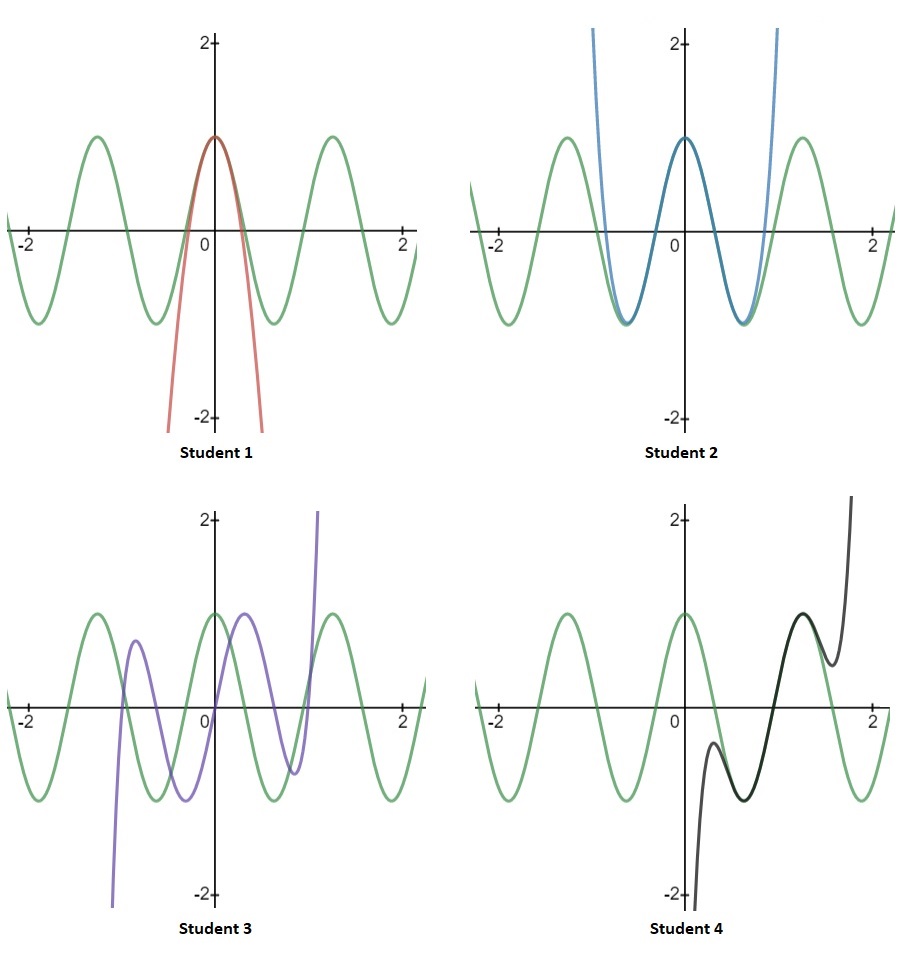
      I believe that Student 1 did the power series expansion for cosine of \(5x\) around \(x=0\) and included terms up to 2nd order because I am only seeing one maximum/minimum in the approximation. (The number of max/mins is one fewer than the highest power in the approximation). Student 1's approximation "appears valid" for \(-0.5<x<0.5\). Outside of that region, the approximation remains concave down, but the original function becomes concave up and then oscillates.

      Student 2 also did a power series expansion for cosine of \(5x\), but I believe they included up to 4th order terms since I see three max/mins. Graphically, the approximation made by Student 2 is reasonably close to the green curve for \(-1<x<1\).

      Student 3 appears to be doing a Taylor approximation for \(\sin(5x)\) instead of cosine, so the series isn't valid for any values of \(x\) even though the function and the power series agree by chance at five isolated points.

      Student 4's approximation seems to be antisymmetric around the point \(x=1\). I conclude the student seems to be using a Taylor series expanded around \(x=1\) instead of \(x=0\), i.e. it is written in terms of powers like \((x-1)^n\). Also, if I want the approximation to be valid within a few percent of the maximum value of the function, then it looks like I can use this approximation in the region from \(x=0.5\) to \(x=1.5\).

4. Sensemaking from Graphs of Power Series I For the following graphs, identify the minimum order in a power series expansion that could accurately describe the curve for all values of the independent variable.

   

   The leftmost graph has 3 turnaround points (maxima and minima) and therefore must, at minimum, be of order 4.

   The middle graph is of \(\sin(x)\) and has an infinite number of maxima and minima. Therefore, it needs an infinite number of power series terms to accurately describe it for all values of \(x\).

   The far right graph appears to be a straight line and so a power series approximation only needs to go to order 1. The first order term is called the "linear" term for this reason.