Avoid: \(2kg\) Instead use: \(2 \text{ kg}\)
There is a space between the number and the unit (the number and the unit are separate “words”). Units are not italicized. This helps distinguish between \(2\text{ kg}\) (two kilograms) and \(2kg\) (\(2\) times \(k\) times \(g\)).
Avoid:10^12, or 1E12 Instead use: \(10^{12}\)
In scientific writing, you have to use superscript. The notation 1E12 is specific to computer coding. The notation 10^12 is a shortcut that might be appropriate for an informal email message.
Avoid:VLED or V_LED or \(V_{LED}\) Instead use: \(V_{\text{LED}}\)
In scientific writing, you have to use subscripts. Note that subscript text such as “LED” is not italicized. In LaTeX you can code this as V_{\text{LED}}. The notation V_LED is a shortcut that might be appropriate for an informal email.
Avoid: wavelength=d*sin(theta) Instead use: \(\lambda=d\sin\theta\)
Algebraic variables are italicized. There are spaces on either side of the equals sign. The sine function is not italic. LaTeX and Microsoft Equation Editor will manage much of this for you.
Avoid: 10 Ohm Instead use: 10 \(\Omega\)
In Microsoft word you can use the font called "Symbol" to get Greek letters. Alternatively, Latex and Microsoft Equation Editor also take care of Greek letters by typing (\Omega).
Avoid: Voltage (v) Instead use: Voltage (V)
Units are case-sensitive. The symbol for the volt unit is capital V.
Avoid: \(\theta = 0.674740942\) Instead use: \(\theta = 0.67\) or \(\theta = 0.675\)
It is unlikely your solution will require more than 1% accuracy.
Algebraic variables are defined in the text the first time they are used.
Use a consistent font size for equations and text.
typography Found in: Contemporary Challenges course(s)
Let's start by visualizing the energy flow associated with driving a gasoline-powered car. We will use a box and arrow diagram, where boxes represent where energy can accumulate, and arrows show energy flow.
The energy clearly starts in the form of gasoline in the tank. Where does it go?
Visualize the energy as an indestructable, incompressible liquid.
“Energy is conserved”
The heat can look like
Hot exhaust gas
The radiator (its job is to dissipate heat)
Friction heating in the drive train
The work contribute to
Rubber tires heated by deformation
Wind, which ultimately ends up as heating the atmosphere
The most important factors for a coarse-grain model of highway driving:
The 75:25 split between “heat” and “work”
The trail of wind behind a car
What might we have missed? Where else might energy have gone?
We ignored the kinetic energy of the car, and the energy dissipated as heat in the brakes. On the interstate this is appropriate, but for city driving the dominant “work” may be in accelerating the car to 30 mph, and with that energy then converted into heat by the brakes.
In rectangular coordinates, the natural unit vectors are \(\{\boldsymbol{\hat x},\boldsymbol{\hat y}\}\), which point in the direction of increasing \(x\) and \(y\), respectively. Similarly, in polar coordinates the natural unit vectors are
\(\boldsymbol{\hat r}\), which points in the direction of increasing \(r\), and \(\boldsymbol{\hat\phi}\), which points in the direction of increasing \(\phi\).
The unit tangent vector to a parametric curve is the unit vector tangent to the curve which points in the direction of increasing parameter. The principal unit normal vector to a parametric curve is the unit vector perpendicular to the curve “in the direction of bending”, which is the direction of the derivative of the unit tangent vector.
Consider the parametric curve
\(\boldsymbol{\vec r} = 3\cos\phi\,\boldsymbol{\hat x} + 3\sin\phi\,\boldsymbol{\hat y}\)
with \(\phi\in[0,2\pi]\). Calculate the unit tangent vector \(\boldsymbol{\hat T}\) and the principal unit normal vector \(\boldsymbol{\hat N}\) for this curve in terms of \(\boldsymbol{\hat x}\) and \(\boldsymbol{\hat y}\).
Consider a circle of radius \(3\) centered at the origin. Determine the unit tangent vector \(\boldsymbol{\hat T}\) and the principal unit normal vector \(\boldsymbol{\hat N}\) for this curve in terms of \(\boldsymbol{\hat r}\) and \(\boldsymbol{\hat\phi}\).
Compare your answers.
Instructor's Guide
Main ideas
Geometric introduction of \(\boldsymbol{\hat r}\) and \(\boldsymbol{\hat\phi}\).
Geometric introduction of unit tangent and normal vectors.
Prerequisites
The position vector \(\vec{r}\).
The derivative of the position vector is tangent to the curve.
Warmup
See the prerequisites. It is possible to briefly introduce these ideas
immediately preceding this activity.
Props
whiteboards and pens
Wrapup
Emphasize that \(\boldsymbol{\hat r}\) and \(\boldsymbol{\hat\phi}\) do not live at the origin! Encourage
students to use the figure provided, which may help alleviate this confusion.
Point out to the students that \(\boldsymbol{\hat r}\) and \(\boldsymbol{\hat\phi}\) are defined everywhere
(except at the origin), whereas \(\boldsymbol{\hat{T}}\) and \(\boldsymbol{\hat{N}}\) are properties of the curve.
It is only on circles that these two notions coincide; \(\boldsymbol{\hat r}\) and \(\boldsymbol{\hat\phi}\) are
adapted to round problems, and circles are round! Symmetry is important.
Emphasize that \(\{\boldsymbol{\hat r},\boldsymbol{\hat\phi}\}\) can be used as a basis (except at the
origin). Point out to the students that their answer to the last problem
gives them a formula expressing \(\boldsymbol{\hat r}\) and \(\boldsymbol{\hat\phi}\) in terms of \(\boldsymbol{\hat{x}}\) and
\(\boldsymbol{\hat{y}}\). When comparing these basis vectors, they should all be drawn with
their tails at the same point.
Details
We have had success helping students master the idea of “direction of
bending” by describing the curve as part of a pickle jar; the principal unit
normal vector points at the pickles!
In the Classroom
The easiest way to find \(\boldsymbol{\hat{N}}\) is to use the dot product to find vectors
orthogonal to \(\boldsymbol{\hat{T}}\), then normalize. Students must then use the “direction
of bending” criterion to choose between the two possible orientations.
Finding \(\boldsymbol{\hat{N}}\) in this way requires the student to give names to the its
unknown components. This is a nontrivial skill; many students will have
trouble with this.
It may be important to draw some examples. Despite that, students still feel wary of embracing \(\boldsymbol{\hat{r}}\) and \(\boldsymbol{\hat{\phi}}\). People will feel more comfortable over the next few classes but emphasize the geometry: the circle is still the circle and the unit tangent remains the same regardless.
Some students are natural geometors and will realize what the desired vectors are. This is terrific. Certainly, it is worthwhile to explicitly demonstrate this, but the point is the geometry can often do the work for you. This will convince students of the value of smart coordinates.
Subsidiary ideas
Dividing any vector by its length yields a unit vector.
Using the dot product to find vectors perpendicular to a given vector.
Homework
Some students will not be comfortable unless they work out the components of
\(\boldsymbol{\hat r}\) and \(\boldsymbol{\hat\phi}\) with respect to \(\boldsymbol{\hat{x}}\) and \(\boldsymbol{\hat{y}}\). Let them.
Enrichment
What units does a unit vector have? Do \(\boldsymbol{\hat r}\) and \(\boldsymbol{\hat\phi}\) have the same
units?
Students, pretending they are point charges, move around the room acting out various prompts from the instructor regarding charge densities, including linear \(\lambda\), surface \(\sigma\), and volume \(\rho\) charge densities, both uniform and non-uniform. The instructor demonstrates what it means to measure these quantities. In a remote setting, we have students manipulate 10 coins to model the prompts in this activity and we demonstrate the answers with coins under a doc cam.
Students, pretending they are point charges, move around the room so as to make an imaginary magnetic field meter register a constant magnetic field, introducing the concept of steady current. Students act out linear \(\vec{I}\), surface \(\vec{K}\), and volume \(\vec{J}\) current densities. The instructor demonstrates what it means to measure these quantities by counting how many students pass through a gate.
A student is invited to “act out” motion corresponding to a plot of effective potential vs. distance. The student plays the role of the “Earth” while the instructor plays the “Sun”.
Students hold rulers and meter sticks to represent a vector field. The instructor holds a hula hoop to represent a small area element. Students are asked to describe the flux of the vector field through the area element.
Students are shown a topographic map of an oval hill and imagine that the classroom is on the hill. They are asked to point in the direction of the gradient vector appropriate to the point on the hill where they are "standing".
The concentration of potassium
\(\text{K}^+\) ions in the internal sap of a plant cell (for example,
a fresh water alga) may exceed by a factor of \(10^4\) the
concentration of \(\text{K}^+\) ions in the pond water in which the
cell is growing. The chemical potential of the \(\text{K}^+\) ions is
higher in the sap because their concentration \(n\) is higher there.
Estimate the difference in chemical potential at \(300\text{K}\) and
show that it is equivalent to a voltage of \(0.24\text{V}\) across the
cell wall. Take \(\mu\) as for an ideal gas. Because the values of the
chemical potential are different, the ions in the cell and in the pond
are not in diffusive equilibrium. The plant cell membrane is highly
impermeable to the passive leakage of ions through it. Important
questions in cell physics include these: How is the high concentration
of ions built up within the cell? How is metabolic energy applied to
energize the active ion transport?
David adds
You might wonder why it is even remotely plausible to consider the
ions in solution as an ideal gas. The key idea here is that the ideal
gas entropy incorporates the entropy due to position dependence, and
thus due to concentration. Since concentration is what differs between
the cell and the pond, the ideal gas entropy describes this pretty
effectively. In contrast to the concentration dependence, the
temperature-dependence of the ideal gas chemical potential will not be
so great.
Students learn about the geometric meaning of the amplitude and period parameters in the sine function. They also practice sketching the sum of two functions by hand.
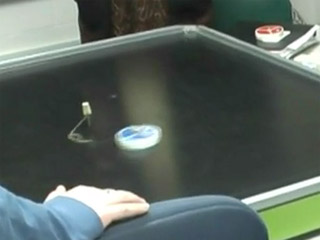
Students observe the motion of a puck tethered to the center of the airtable. Then they plot the potential energy for the puck on their small whiteboards. A class discussion follows based on what students have written on their whiteboards.
Consider an air hockey puck of mass \(m\)
tethered to a peg in the middle of an air hockey table.
The tether is made from a small piece of thread of length \(L\). You give the
puck a push so that its initial
angular momentum is \(\ell\),
Briefly explain why this is a central force system.
A central force problem involves two objects. Find an approximate formula for the reduced mass of this central force system and explain briefly, in words, why this makes sense.
Make a sketch of the potential energy of this system plotted vs. \(r\), the distance from the peg.
Recall that the effective potential is the SUM of the potential (the one you just plotted!!!) and the kinetic energy due to the angular part of the motion.
\[U_{\text{eff}}=U(r)+\frac{\ell^2}{2\mu r^2}\]
Make a sketch of the effective potential.
Briefly discuss the possible orbit shapes that can arise from this effective potential.
How should you push the puck to establish a circular orbit?
(i.e. give the initial position and direction of push).
(Messy algebra) Convince yourself that the expressions for kinetic energy in original and center of mass coordinates are equivalent. The same for angular momentum.
Consider a system of two particles of mass \(m_1\) and \(m_2\).
Show that the total kinetic energy of the system is the same as that of two
“fictitious” particles: one of mass \(M=m_1+m_2\) moving with the velocity of the
center of mass and one of mass \(\mu\) (the reduced mass) moving with the
velocity of the relative position.
Show that the total angular momentum of the system can similarly be decomposed
into the angular momenta of these two fictitious particles.
We will show that the components of the angular momentum operator \(\vec{L}\), written in
differential operator form in rectangular components, satisfy the commutation
relations:
\begin{equation}
\left[L_x,L_y\right]=+i\hbar L_z \qquad(\text{and cyclic permutations})
\end{equation}
First calculate the components of angular momentum classically:
\begin{align}
\vec{L}&=\vec{r}\times\vec{p}\\
&=(x\hat{x}+y\hat{y}+z\hat{z})\times(p_x\hat{x}+p_y\hat{y}+p_z\hat{z})\\
&=(yp_z-zp_y)\hat{x}+(zp_x-xp_z)\hat{y}+(xp_y-yp_x)\hat{z}
\end{align}
Making the standard quantum substitutions,
\begin{align}
p_x&\rightarrow -i\hbar\partial_x\\
p_y&\rightarrow -i\hbar\partial_y\\
p_z&\rightarrow -i\hbar\partial_z\\
\end{align}
we obtain the following operators for the components of angular momentum:
\begin{align}
\hat{L}_x&=-i\hbar(y\partial_z-z\partial_y)\\
\hat{L}_y&=-i\hbar(z\partial_x-x\partial_z)\\
\hat{L}_z&=-i\hbar(x\partial_y-y\partial_x)\\
\end{align}
To see the role of the product rule in the commutation relations, it is helpful to give the partial derivatives an arbitrary function \(\psi\) to act on.
\begin{align}
\left[\hat{L}_x,\hat{L}_y\right]\psi
&=\left[-i\hbar(y\partial_z-z\partial_y),
-i\hbar(z\partial_x-x\partial_z)\right]\psi\\
&=-\hbar^2\left\{(y\partial_z-z\partial_y)(z\partial_x-x\partial_z)
-(z\partial_x-x\partial_z)(y\partial_z-z\partial_y)\right\}\psi
\end{align}
Now, foil-like-mad. Make sure that all of the partial derivatives act on EVERYTHING to their right. Two of the terms above of the form
\begin{align}
y\,\partial_z(z\,\partial_x \psi)
\end{align}
require a product rule:
\begin{align}
y\,\partial_z(z\,\partial_x \psi)
&=y((\partial_z z)(\partial_x\psi)+z(\partial_x\partial_x\psi))\\
&=y\partial_x\psi+yz(\partial_x\partial_x\psi)
\end{align}
Continuing the calculation above, we see that
all of the second derivative terms will cancel because the order of differentiation doesn't matter, leaving only the first derivative terms from the product rule.
\begin{align}
\left[\hat{L}_x,\hat{L}_y\right]\psi
&=\left[-i\hbar(y\partial_z-z\partial_y),
-i\hbar(z\partial_x-x\partial_z)\right]\psi\\
&=-\hbar^2\left\{(y\partial_z-z\partial_y)(z\partial_x-x\partial_z)
-(z\partial_x-x\partial_z)(y\partial_z-z\partial_y)\right\}\psi\\
&=-\hbar^2\left\{\left(y\,\partial_z(z\,\partial_x \psi)
-y\,\partial_z(x\,\partial_z \psi)
-z\,\partial_y(z\,\partial_x \psi)
+z\,\partial_y(x\,\partial_z \psi)\right)\right.\\
&\;\;\;\quad\quad\left.-\left(z\,\partial_x(y\,\partial_z \psi)
-z\,\partial_x(z\,\partial_y \psi)
-x\,\partial_z(y\,\partial_z \psi)
+x\,\partial_z(z\,\partial_y \psi)\right)
\right\}\\
&=-\hbar^2\left\{\left(\cancel{yz(\partial_z\partial_x\psi)}
+y\partial_x\psi
-\cancel{yx(\partial_z^2\psi)}
-\cancel{z^2(\partial_y\partial_x\psi)}
+\cancel{zx(\partial_y\partial_z\psi)}\right)\right.\\
&\;\;\;\quad\quad\left.-\left(\cancel{zy(\partial_x\partial_z\psi)}
-\cancel{z^2(\partial_x\partial_y\psi)}
-\cancel{xy(\partial_z^2\psi)}
+\cancel{xz(\partial_z\partial_y\psi)}
+x\partial_y\psi\right)
\right\}\\
&=i\hbar\left(-i\hbar(-y\partial_x+x\partial_y)\psi\right)\\
&=i\hbar\hat{L}_z\, \psi
\end{align}
The other components are cyclic permutations of this calculation.
Let's apply the relationship of heat, entropy, and temperature to a contemporary challenge!
We'd like to maximize the efficiency of any process that is based on heat flow as an input.
Just a few examples of heat engines.
Energy flow diagram
Energy flow diagram
The efficiency of the machine is
\begin{align}
\text{efficiency} &= \frac{W}{Q_{\text{in}}}
\\
\textit{e.g.} &=\frac{500\text{ J}}{1000\text{ J}} = 50\%
\end{align}
For a car engine, \(T_H\approx 600\text{ K}\) and \(T_C\approx 300\text{ K}\).
Remember that \(\Delta S=\frac{Q}{T}\), and \(\Delta S_{\text{tot}} \ge 0\).
In this activity, students apply the Stefan-Boltzmann equation and the principle of energy balance in steady state to find the steady state temperature of a black object in near-Earth orbit.
Google “phet blackbody spectrum”' and open the simulation.
At what wavelength is the peak in spectral intensity
\(\lambda_{\text{peak}}\) for a black rock on the Earth's surface,
\(\lambda_{\text{peak}}\) for the black walls of a pizza oven,
\(\lambda_{\text{peak}}\) for a light bulb,
\(\lambda_{\text{peak}}\) for the sun.
Check that the peak wavelength decreases with temperature following a \(1/T\) relationship.
Use the numerical integration feature (the checkbox labelled “intensity” near the upper-right corner of the graph) to find the total intensity, in units of \(\text{W/m}^2\), emitted by
a black rock on the Earth's surface,
the black walls of a pizza oven,
the surface of a tungsten light bulb filament,
the surface of the sun.
Check that these intensities are proportional to \(T^4\). Note, the quick way to check involves ratios: Does \(\frac{I_1}{I_2} = \left(\frac{T_1}{T_2}\right)^4\)?
How cold should you make an object if you want zero thermal radiation emitted?
(Extra---if your group has time)
For an incandescent light bulb with a filament surface area of \(A\), estimate how efficiently it converts electrical energy into visible photons. Hint: you will need to estimate the following ratio:
\begin{align*}
\frac{\text{Electromagnetic radiation in visible wavelengths}}{
\text{Total electromagnetic radiation}
} = \frac{
A\int_{400\text{ nm}}^{700\text{ nm}} S_\lambda(\lambda, T)d\lambda
}{
A\int_{0}^{\infty} S_\lambda(\lambda, T)d\lambda
}
\end{align*}
Estimate the filament surface area \(A\) for a 60 W light bulb.
blackbody Found in: Contemporary Challenges course(s)
These notes, from the third week of https://paradigms.oregonstate.edu/courses/ph441 cover the canonical ensemble and Helmholtz free energy. They include a number of small group activities.
Students solve for the equations of motion of a box sliding down (frictionlessly) a wedge, which itself slides on a horizontal surface, in order to answer the question "how much time does it take for the box to slide a distance \(d\) down the wedge?". This activities highlights finding kinetic energies when the coordinate system is not orthonormal and checking special cases, functional behavior, and dimensions.
In your kits for the Portable Partial Derivative Machine should be the following:
A 1ft by 1ft board with 5 holes and measuring tapes (the measuring tapes will be on the top side)
2 S-hooks
A spring with 3 strings attached
2 small cloth bags
4 large ball bearings
8 small ball bearings
2 vertical clamp pulleys
A ziploc bag containing
5 screws
5 hex nuts
5 washers
5 wing nuts
2 horizontal pulleys
To assemble the Portable PDM, start by placing the PDM on a table surface with the measuring tapes perpendicular to the table's edge and the board edge with 3 holes closest to you.
one screw should be put through each hole so that the threads stick out through the top side of the board. Next use a hex nut to secure each screw in place. It is not critical that they be screwed on any more than you can comfortably manage by hand.
After securing all 5 screws in place with a hex nut, put a washer on each screw.
Slide a horizontal pulley onto screws 1 and 2 (as labeled above).
On all 5 screws, add a wing nut to secure the other pieces. Again, it does not need to be tightened all the way as long as it is secure enough that nothing will fall off.
Using the middle wingnut/washer/screw (Screw 4), clamp the shortest of the strings tied to the spring.
Loop the remaining 2 looped-ends of string around the horizontal pulleys and along the measuring tape.
Using the string as a guide, clamp the vertical pulleys into place on the edge of the board.
Through the looped-end of each string, place 1 S-hook.
Put the other end of each s-hook through the hole in the small cloth bag.
Here is a poor photo of the final result, which doesn't show the two vertical pulleys. If you would like, you could view a video of the building process.
PDM Found in: Energy and Entropy, None course(s)Found in: The Partial Derivatives Machine sequence(s)
Students are placed into small groups and asked to calculate the total differential of a function of two variables, each of which is in turn expressed in terms of two other variables.
This activity starts with a brief lecture introduction to power series and a short derivation of the formula for calculating the power series coefficients.
\[c_n={1\over n!}\, f^{(n)}(z_0)\]
Students use this formula to compute the power series coefficients for a \(\sin\theta\) (around both the origin and (if time allows) \(\frac{\pi}{6}\)). The meaning of these coefficients and the convergence behavior for each approximation is discussed in the whole-class wrap-up and in the follow-up activity: Visualization of Power Series Approximations.
Taylor SeriesCoefficentsPower Series Found in: Theoretical Mechanics, AIMS Maxwell, Static Fields, Problem-Solving, None course(s)Found in: Power Series Sequence (Mechanics), Power Series Sequence (E&M) sequence(s)
Calculate based on the Clausius-Clapeyron equation the value of
\(\frac{dT}{dp}\) near \(p=1\text{atm}\) for the liquid-vapor
equilibrium of water. The heat of vaporization at
\(100^\circ\text{C}\) is \(2260\text{ J g}^{-1}\). Express the result
in kelvin/atm.
In carbon monoxide
poisoning the CO replaces the \(\textsf{O}_{2}\) adsorbed on
hemoglobin (\(\text{Hb}\)) molecules in the blood. To show the effect,
consider a model for which each adsorption site on a heme may be
vacant or may be occupied either with energy \(\varepsilon_A\) by one
molecule \(\textsf{O}_{2}\) or with energy \(\varepsilon_B\) by one
molecule CO. Let \(N\) fixed heme sites be in equilibrium with
\(\textsf{O}_{2}\) and CO in the gas phases at concentrations such
that the activities are \(\lambda(\text{O}_2) = 1\times 10^{-5}\) and
\(\lambda(\text{CO}) = 1\times 10^{-7}\), all at body temperature
\(37^\circ\text{C}\). Neglect any spin multiplicity factors.
First consider the system in the absence of CO. Evaluate
\(\varepsilon_A\) such that 90 percent of the \(\text{Hb}\) sites
are occupied by \(\textsf{O}_{2}\). Express the answer in eV per
\(\textsf{O}_{2}\).
Now admit the CO under the specified conditions. Fine
\(\varepsilon_B\) such that only 10% of the Hb sites are occupied
by \(\textsf{O}_{2}\).
The center-of-mass motion is determined by the net external force, even when the particles are not interacting. Practice with center-of-mass coordinates.
Consider two particles of equal mass \(m\). The forces on the
particles are \(\vec F_1=0\) and \(\vec F_2=F_0\hat{x}\) (for this problem, ignore gravitational forces between the two particles). If the
particles are initially at rest at the origin, find the position,
velocity, and acceleration of the center of mass as functions of
time. Solve this problem in two ways,
solve for the motion of each of the particles, separately,
then see what happens to the center of mass
solve directly for the center of mass motion
Write a short description
comparing the two solutions.
(Quick) Purpose: Recognize the definition of a central force. Build experience about which common physical situations represent central forces and which don't.
Which of the following forces can be central forces? which cannot? If the force CAN be a central force, explain the circumstances that would allow it to be a central force.
The force on a test mass \(m\) in a gravitational field \(\vec{g~}\),
i.e. \(m\vec g\)
The force on a test charge \(q\) in an electric field \(\vec E\), i.e.
\(q\vec E\)
The force on a test charge \(q\) moving at velocity \(\vec{v~}\) in a
magnetic field \(\vec B\), i.e. \(q\vec v \times \vec B\)
In this course, we will examine a mathematically tractable and physically useful problem - that of two bodies interacting with each other through a central force, i.e. a force that has two characteristics:
Definition of a Central Force:
A central force depends only on the separation distance between the two bodies,
A central force points along the line connecting the two bodies.
The most common examples of this type of force are those that have \(\frac{1}{r^2}\) behavior, specifically the Newtonian gravitational force between two point (or spherically symmetric) masses and the Coulomb force between two point (or spherically symmetric) electric charges. Clearly both of these examples are idealizations - neither ideal point masses or charges nor perfectly spherically symmetric mass or charge distributions exist in nature, except perhaps for elementary particles such as electrons. However, deviations from ideal behavior are often small and can be neglected to within a reasonable approximation. (Power series to the rescue!)
Also, notice the difference in length scale: the archetypal gravitational example is planetary motion - at astronomical length scales; the archetypal Coulomb example is the hydrogen atom - at atomic length scales.
The two solutions to the central force problem - classical behavior exemplified by the gravitational interaction and quantum behavior exemplified by the Coulomb interaction - are quite different from each other.
By studying these two cases together in the same course, we will be able to explore the strong similarities and the important differences between classical and quantum physics.
Two of the unifying themes of this topic are the conservation laws:
Conservation of Energy
Conservation of Angular Momentum
The classical and quantum systems we will explore both have versions of these conservation laws, but they come up in the mathematical formalisms in different ways.
You should have covered energy and angular momentum in your introductory physics course, at least in simple, classical mechanics cases. Now is a great time to review the definitions of energy and angular momentum, how they enter into dynamical equations (Newton's laws and kinetic energy, for example), and the conservation laws.
In the classical mechanics case, we will obtain the equations of motion in three equivalent ways,
using Newton's second law,
using Lagrangian mechanics,
using energy conservation.
so that you will be able to compare and contrast the methods.
The Newtonian approach is the most straightforward and naive, but it
suggests changes of coordinates that inform the other methods. The Lagrangian
and energy conservation approaches are slightly more sophisticated in that they exploit more of the symmetries from the beginning.
We will also consider forces that depend on the distance between the two bodies in ways other than \(\frac{1}{r^2}\) and explore the kinds of motion they produce.
A circular cylinder of radius \(R\)
rotates about the long axis with angular velocity \(\omega\). The
cylinder contains an ideal gas of atoms of mass \(M\) at temperature
\(T\). Find an expression for the dependence of the concentration
\(n(r)\) on the radial distance \(r\) from the axis, in terms of
\(n(0)\) on the axis. Take \(\mu\) as for an ideal gas.
This small group activity is designed to provide practice with the chain rule and to develop familiarity with polar coordinates.
Students work in small groups to relate partial derivatives in rectangular and polar coordinates.
The whole class wrap-up discussion emphasizes the importance of specifying what quantities are being held constant.
This small group activity using surfaces combines practice with the multivariable chain rule while emphasizing numerical representations of derivatives.
Students work in small groups to measure partial derivatives in both rectangular and polar coordinates, then verify their results using the chain rule.
The whole class wrap-up discussion emphasizes the relationship between a directional derivative in the \(r\)-direction and derivatives in \(x\)- and \(y\)-directions using the chain rule.
Consider the region \(D\) in the \(xy\)-plane shown below, which is bounded by
\[u=9 \qquad u=36 \qquad v=1 \qquad v=4\]
where
\[u=xy \qquad v={y\over x}\]
If you want to determine \(x\) and \(y\) as functions of \(u\) and \(v\), consider
\(uv\) and \(u/v\).
List as many methods as you can think of for finding the area of the given
region.
It is enough to refer to the methods by name or describe them briefly.
For at least 3 of these methods, give explicitly the formulas you would use to
find the area.
You must put limits on your integrals, but you do not need to evaluate
them.
Using any 2 of these methods, find the area.
One of these should be a method we have learned recently.
Now consider the following integral over the same region \(D\):
\(\int\!\!\int_D {y\over x} \>\>dA\)
Which of the above methods can you use to do this integral?
Do the integral.
Main ideas
There are many ways to solve this problem!
Using Jacobians (and inverse Jacobians)
Prerequisites
Surface integrals
Jacobians
Green's/Stokes' Theorem
Warmup
Perhaps a discussion of single and double integral techniques for solving this
problem.
Props
whiteboards and pens
Wrapup
This is a good conclusion to the course, as it reviews many integration
techniques. We emphasize that (2-dimensional) change-of-variable problems are
a special case of surface integrals.
Here are some of the methods one could use to do these integrals:
change of variables (at least 2 ways)
Area Corollary to Green's Theorem (at least 2 ways)
ordinary single integral (at least 2 ways)
ordinary double integral (at least 2 ways)
surface integral
Details
In the Classroom
Some students will want to simply use Jacobian formulas; encourage such
students to try to solve this problem both by computing
\(\frac{\partial(x,y)}{\partial(u,v)}\) and by computing \(\frac{\partial(u,v)}{\partial(x,y)}\).
Other students will want to work directly with \(d\boldsymbol{\vec{r}}_1\) and \(d\boldsymbol{\vec{r}}_2\). This
works fine if one first solves for \(x\) and \(y\) in terms of \(u\) and \(v\).
Students who compute \(d\boldsymbol{\vec{r}}_1\) and \(d\boldsymbol{\vec{r}}_2\) directly can easily get confused,
since they may try to eliminate \(x\) or \(y\), rather than \(u\) or \(v\).
Along the curve \(v=\hbox{constant}\), one has \(dy=v\,dx\), so that
\(d\boldsymbol{\vec{r}}_1 = dx\,\boldsymbol{\hat{x}} + dy\,\boldsymbol{\hat{y}} = (\boldsymbol{\hat{x}} + v\,\boldsymbol{\hat{y}})\,dx\),
which some students will want to write in terms of \(x\) alone. But one needs
to express this in terms of \(du\)! This can be done using
\(du = x\,dy + y\,dx = x (v\,dx) + y\,dx = 2y\,dx\),
so that
\(d\boldsymbol{\vec{r}}_1 = (\boldsymbol{\hat{x}} + v\,\boldsymbol{\hat{y}}) \,\frac{du}{2y}\).
A similar argument leads to
\(d\boldsymbol{\vec{r}}_2 = (-\frac{1}{v}\,\boldsymbol{\hat{x}}+\boldsymbol{\hat{y}})\,\frac{x\,dv}{2}\) for \(u=\hbox{constant}\),
so that
\(d\boldsymbol{\vec{S}}
= d\boldsymbol{\vec{r}}_1\times d\boldsymbol{\vec{r}}_2
= \boldsymbol{\hat{z}} \,\frac{x}{2y}\,du\,dv
= \boldsymbol{\hat{z}} \,{du\,dv\over2v}\).
This calculation can be done without solving for \(x\) and \(y\), provided one
recognizes \(v\) in the penultimate expression.
Emphasize that one must choose parameters, both on the region, and on each
curve, and that \(u\) and \(v\) are chosen to make the limits easy.
Take time before the activity to gauge students' recollection of single variable techniques and the Jacobian. After the activity, be sure to set up more than one approach. People will be fine after the first couple of steps but shouldn't leave class feeling stuck.
Subsidiary ideas
Review of Green's Theorem
Review of single integral techniques
Review of double integral techniques
Enrichment
Discuss the 3-dimensional case, perhaps relating it to volume integrals.
Students consider the change in internal energy during three different processes involving a container of water vapor on a stove. Using the 1st Law of Thermodynamics, students reason about how the internal energy would change and then compare this prediction with data from NIST presented as a contour plot.
Students use a plastic surface representing the potential due to a charged sphere to explore the electrostatic potential, equipotential lines, and the relationship between potential and electric field.


(b)
(c)
(d)


