Activities and Homework Problems

None

Use the formula for a Taylor series: \[f(z)=\sum_{n=0}^{\infty} \frac{1}{n!} \frac{d^n f(a)}{dz^n} (z-a)^n\] to find the series expansion for \(f(z)=\cos(kz)\) to second order around \(z=2\).

1. Simplify the following expressions:

   1. \(\ln{x}+\ln{y}\)

   2. \(\ln{a}-\ln{b}\)

   3. \(2\ln{f}+3\ln{f}\)

   4. \(e^{m}e^{k}\)

   5. \(\frac{e^{c}}{e^{d}}\)

2. Expand the following expressions:

   1. \(e^{(3h-j)}\)

   2. \(e^{2(c+w)}\)

   3. \(\ln{h/g}\)

   4. \(\ln(kT)\)

   5. \(\ln{\sqrt{\frac{q}{r}}}\)

Write out the terms in the following sums that have the lowest energy. Stop when you have at least 9 terms, but only stop at some point that is logical, given the symmetries and degeneracies. Briefly explain why you chose to stop when you did. You may have to guess what system you are working from the form of the sum and which eigenvalue(s) determine the energy. You may assume that low energies correspond to eigenvalues near zero. Clearly state any assumptions that you make. You may use bra/ket notation in your solutions. (If these directions are unclear, check out the solutions below for some examples.)

1. \[\sum_{m=-\infty}^{\infty} c_m e^{im\phi}\]
2. \[\sum_{m=1}^{\infty}\sum_{n=1}^{\infty} c_{mn} \sin\left(\frac{m\pi x}{L_x}\right)\sin\left(\frac{n\pi y}{L_y}\right)\]
3. \[\sum_{n=1}^{\infty}\sum_{\ell=0}^{n-1}\sum_{m=-\ell}^{\ell} c_{n \ell m} \left|{n, \ell, m}\right\rangle \]

As discussed in class, we can consider a black body as a large box with a small hole in it. If we treat the large box a metal cube with side length \(L\) and metal walls, the frequency of each normal mode will be given by: \begin{align} \omega_{n_xn_yn_z} &= \frac{\pi c}{L}\sqrt{n_x^2 + n_y^2 + n_z^2} \end{align} where each of \(n_x\), \(n_y\), and \(n_z\) will have positive integer values. This simply comes from the fact that a half wavelength must fit in the box. There is an additional quantum number for polarization, which has two possible values, but does not affect the frequency. Note that in this problem I'm using different boundary conditions from what I use in class. It is worth learning to work with either set of quantum numbers. Each normal mode is a harmonic oscillator, with energy eigenstates \(E_n = n\hbar\omega\) where we will not include the zero-point energy \(\frac12\hbar\omega\), since that energy cannot be extracted from the box. (See the Casimir effect for an example where the zero point energy of photon modes does have an effect.)

Note

This is a slight approximation, as the boundary conditions for light are a bit more complicated. However, for large \(n\) values this gives the correct result.

1. Show that the free energy is given by \begin{align} F &= 8\pi \frac{V(kT)^4}{h^3c^3} \int_0^\infty \ln\left(1-e^{-\xi}\right)\xi^2d\xi \\ &= -\frac{8\pi^5}{45} \frac{V(kT)^4}{h^3c^3} \\ &= -\frac{\pi^2}{45} \frac{V(kT)^4}{\hbar^3c^3} \end{align} provided the box is big enough that \(\frac{\hbar c}{LkT}\ll 1\). Note that you may end up with a slightly different dimensionless integral that numerically evaluates to the same result, which would be fine. I also do not expect you to solve this definite integral analytically, a numerical confirmation is fine. However, you must manipulate your integral until it is dimensionless and has all the dimensionful quantities removed from it!

2. Show that the entropy of this box full of photons at temperature \(T\) is \begin{align} S &= \frac{32\pi^5}{45} k V \left(\frac{kT}{hc}\right)^3 \\ &= \frac{4\pi^2}{45} k V \left(\frac{kT}{\hbar c}\right)^3 \end{align}

3. Show that the internal energy of this box full of photons at temperature \(T\) is \begin{align} \frac{U}{V} &= \frac{8\pi^5}{15}\frac{(kT)^4}{h^3c^3} \\ &= \frac{\pi^2}{15}\frac{(kT)^4}{\hbar^3c^3} \end{align}

For \(\ell=1\), the operators that measure the three components of angular momentum in matrix notation are given by: \begin{align} L_x&=\frac{\hbar}{\sqrt{2}}\left( \begin{matrix} 0&1&0\\ 1&0&1\\ 0&1&0 \end{matrix} \right)\\ L_y&=\frac{\hbar}{\sqrt{2}}\left( \begin{matrix} 0&-i&0\\ i&0&-i\\ 0&i&0 \end{matrix} \right)\\ L_z&=\;\;\;\hbar\left( \begin{matrix} 1&0&0\\ 0&0&0\\ 0&0&-1 \end{matrix} \right) \end{align}

Show that:

1. Find the commutator of \(L_x\) and \(L_y\).
2. Find the matrix representation of \(L^2=L_x^2+L_y^2+L_z^2\).
3. Find the matrix representations of the raising and lowering operators \(L_{\pm}=L_x\pm iL_y\). (Notice that \(L_{\pm}\) are NOT Hermitian and therefore cannot represent observables. They are used as a tool to build one quantum state from another.)
4. Show that \([L_z, L_{\pm}]=\lambda L_{\pm}\). Find \(\lambda\). Interpret this expression as an eigenvalue equation. What is the operator?
5. Let \(L_{+}\) act on the following three states given in matrix representation. \begin{equation} \left|{1,1}\right\rangle =\left( \begin{matrix} 1\\0\\0 \end{matrix} \right)\qquad \left|{1,0}\right\rangle =\left( \begin{matrix} 0\\1\\0 \end{matrix} \right)\qquad \left|{1,-1}\right\rangle =\left( \begin{matrix} 0\\0\\1 \end{matrix} \right) \end{equation} Why is \(L_{+}\) called a “raising operator”?

Instructor's Guide

Introduction

This activity is meant to lay the foundation of what raising and lowering oporators are and how they can be used. This material will become very important for students' study of symmetry matrices in PH427 and the Quantum Harmonic Oscillator in the Quantum Capstone.

Student Conversations

At this stage, students will not have seen commutators or done much matrix multiplication in a while, so students may progress lower here than you'd expect. It will be important for the teaching team to be on the look out for groups that are confused at the beginning since some will forget that a commutator can have the form \([A,B]=AB-BA\), which is necessary to progress.

Making sure the teaching team has a good handle on the results of each calculation so they can help trouble shoot errors made during matrix multiplication which are hard to catch in the act and usually can most easilty be inferred from an erronous result (which the students themselves won't usually recognize).

Wrap-up

It is a good idea to reinforce the patterns seen in orbital angular momentum to their experiences with spin angular momentum, such as that cross product-like relationship between commutators of cartesian directed angular momenta. Then it becomes easy to contrast those patterns with that of the raising and lower operators and emphasize that these are not observables which correspond to measures of angular momentum but a different object entirely.

While their importance should be emphasized for study of periodic systems and the quantum harmonic oscilator, it should also be mentioned these operators will not be a major focus of this course or our study of the Hydrogen atom as we head into the home stretch of the course. This content is largely a very important detour.

Using your favorite graphing package, make a plot of the reduced mass \begin{equation} \mu=\frac{m_1\, m_2}{m_1+m_2} \end{equation} as a function of \(m_1\) and \(m_2\). What about the shape of this graph tells you something about the physical world that you would like to remember? You should be able to find at least three things. Hint: Think limiting cases.

In this small group activity, students draw components of a vector in Cartesian and polar bases. Students then write the components of the vector in these bases as both dot products with unit vectors and as bra/kets with basis bras.

None

Representations of the Infinite Square Well

Consider three particles of mass \(m\) which are each in an infinite square well potential at \(0<x<L\).

The energy eigenstates of the infinite square well are:

\[ \left\langle {x}\middle|{E_n}\right\rangle =\phi_n(x) = \sqrt{\frac{2}{L}}\sin{\left(\frac{n \pi x}{L}\right)}\]

with energy eigenvalues \(E_n = \frac{n^2 \pi^2 \hbar^2}{2mL^2}\)

The particles are initially in the states, respectively: \begin{eqnarray*} |\psi_a(0)\rangle &=& A \Big[\left|{E_1}\right\rangle + 2i \left|{E_4}\right\rangle - 3\left|{E_{10}}\right\rangle \Big]\\[6pt] \psi_b(x,0) &=& B \left[\sqrt{\frac{2}{L}}\sin{\left(\frac{\pi x}{L}\right)} + i \sqrt{\frac{8}{L}}\sin{\left(\frac{4\pi x}{L}\right)} - \sqrt{\frac{18}{L}}\sin{\left(\frac{10\pi x}{L}\right)} \right]\\[6pt] \psi_c(x,0) &=& C x(x-L) \end{eqnarray*}

For each particle:

1. Determine the value of the normalization constant.
2. At \(t=0\), what is the probability of measuring the energy of the particle to be \(\frac{8\pi^2\hbar^2}{mL^2}\)?
3. Find the state of the particle at a later time \(t\).
4. What is the probability of measuring the energy of the particle to be the same value \(\frac{8\pi^2\hbar^2}{mL^2}\) at a later time \(t\)?
5. What is the probability of finding the particle to be in the left half of the well?

Student Conversations

1. Help students recognize that particle \(a\) and particle \(b\) are in the same state.
2. For normalization, emphasize that you must calculate the square of the norm of the state BEFORE you integrate.
3. The energy value given is simplified - students need to recognize that this energy corresponds to \(n=4\).
4. Time evolving particle \(c\) is brutal for the students. Reassure students that they have to leave it as a sum. Setting up the integral is the point here. For time expediancy, encourage students to leave the integral to be evaluated later.
5. For Hamiltonian's that don't don't depend on time, the probabilities of measuring energies are time independent.
6. Emphasize to students that you can't calculate the probability of finding a particle in a region in Dirac notation.

Students each recall a representation of vectors that they have seen before and record it on an individual whiteboard. The instructor uses these responses to generate a whole class discussion that compares and contrasts the features of the representations. If appropriate for the class, the instructor introduces bra/ket notation as a new, but valuable representation.

These are notes, essentially the equation sheet, from the final review session for https://paradigms.oregonstate.edu/courses/ph441.

Students take the inner product of vectors that lie on the spacetime axis to show that they are orthogonal. To do the inner product, students much use the Minkowski metric.

None

None

None

• How to find area, and volume elements in curvilinear coordinates using geometric methods.

Consider a very light particle of mass \(\mu\) scattering from a very heavy, stationary particle of mass \(M\). The force between the two particles is a repulsive Coulomb force \(\frac{k}{r^2}\) (neglect the gravitational force). The impact parameter \(b\) in a scattering problem is defined to be the distance which would be the closest approach if there were no interaction (See Figure). The initial velocity (far from the scattering event) of the mass \(\mu\) is \(\vec v_0\).

Answer the following questions about this situation in terms of \(k\), \(M\), \(\mu\), \(\vec v_0\), and \(b\). (It is not necessarily wise to answer these questions in order.)

1. What is the initial angular momentum of the system?
2. What is the initial total energy of the system?
3. What is the distance of closest approach \(r_{\rm{min}}\) with the interaction?
4. Sketch the effective potential.
5. What is the angular momentum at \(r_{\rm{min}}\)?
6. What is the total energy of the system at \(r_{\rm{min}}\)?
7. What is the radial component of the velocity at \(r_{\rm{min}}\)?
8. What is the tangential component of the velocity at \(r_{\rm{min}}\)?
9. What is the value of the effective potential at \(r_{\rm{min}}\)?
10. For what values of the initial total energy are there bound orbits?
11. Using your results above, write a short essay describing this type of scattering problem, at a level appropriate to share with another Paradigm student.

1. Set-Up a Sequential Measurement

   1. Add an analyzer to the experiment by:

      1. Break the links between the analyzer and the counters by clicking on the boxes with up and down arrow labels on the analyzer.
      2. Click and drag a new connection from the analyzer to empty space to create a new element. A new analyzer is one of the options.

   2. Measure \(S_z\) twice in succession.

      

      What is the probability that a particle leaving the first analyzer with \(S_z=\frac{+\hbar}{2}\) will be measured by the second analyzer to have \(S_z=\frac{-\hbar}{2}\)?

   3. Set the first analyzer to measure \(S_z\) and the second analyzer to measure \(S_x\).

      

      What have you learned from these experiments?

   
   

2. Try All Combinations of Sequential Measurements

   In the table, enter the probability of a particle exiting the 2nd analyzer with the spin indicated in row if the particle enters the 2nd analyzer with the spin indicated in each column.

   

   
   

3. You can rotate the Stern-Gerlach analyzers to any direction you want (using spherical coordinates).

   Choose an arbitrary direction (not along one of the coordinate axes) for the 1st analyzer and measure the spin along the coordinate directions for the 2nd analyzer.

   

None

Write out the first four nonzero terms in the series:

1. \[\sum\limits_{n=0}^\infty \frac{1}{n!}\]

2. \[\sum\limits_{n=1}^\infty \frac{(-1)^n}{n!}\]
3. \begin{equation} \sum\limits_{n=0}^\infty {(-2)^{n}\,\theta^{2n}} \end{equation}

Write (a good guess for) the following series using sigma \(\left(\sum\right)\) notation. (If you only know a few terms of a series, you don't know for sure how the series continues.)

1. \[1 - 2\,\theta^2 + 4\,\theta^4 - 8\,\theta^6 +\,\dots\]

2. \[\frac14 - \frac19 + \frac{1}{16} - \frac{1}{25}+\,\dots\]

Use the power series method to solve Legendre's Equation \begin{equation} \frac{d^2 P}{d z^2} -\frac{2z}{1-z^2}\frac{d P}{d z} -\frac{A}{1-z^2} P=0 \label{legendrepolyeqn} \end{equation}

Students compute inner products to expand a wave function in a sinusoidal basis set. This activity introduces the inner product for wave functions, and the idea of approximating a wave function using a finite set of basis functions.

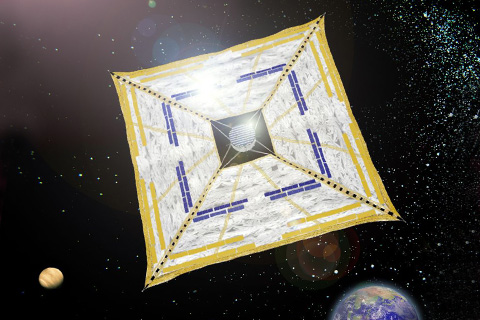
The first spacecraft using a solar sail for propulsion was launched in 2010. Its name is IKAROS. It has a square sail with dimensions 14 m x 14 m. Assume that the sail's mass is 2 kg and it reflects 100% of incident photons. When IKAROS is loaded with other equipment, the total mass of the vehicle is 10 kg. The sail is orientated to receive maximum light from the sun.

1. Calculate the momentum of the photons that come from the sun and hit the solar sail in 1 second. Assume a solar intensity of 1300 J/(s.m\(^2\)).
2. How much momentum will be transferred from solar photons to IKAROS in one day? Give a numerical answer in units of kg.m/s (assume a constant solar intensity).
3. What is the change in the solar sail's velocity in one day? (assume that acceleration is only caused by sunlight).

None

None

\(\boxed{\begin{array}{lll} \ell& m & \quad\quad\quad\; Y_\ell^m(\theta,\phi) \\[.35cm] \hline \\[.03cm] 0 & 0 & \quad\;\; Y_0^0=\sqrt{\frac{1}{4\pi}} \\[.35cm] 1 & 0 & \quad\;\; Y_1^0=\sqrt{\frac{3}{4\pi}}\cos\theta \\[.35cm] & \pm1 & \quad Y_1^{\pm1}=\mp\sqrt{\frac{3}{8\pi}}\sin\theta e^{\pm i\phi} \\[.35cm] 2 & 0 & \quad\;\;Y_2^0=\sqrt{\frac{5}{16\pi}}\left(3\cos^2\theta-1 \right) \\[.35cm] & \pm1 & \quad Y_2^{\pm1}=\mp\sqrt{\frac{15}{8\pi}}\sin\theta\cos \theta e^{\pm i\phi} \\[.35cm] & \pm2 & \quad Y_2^{\pm2}=\sqrt{\frac{15}{32\pi}}\sin^2\theta e^{\pm2i\phi} \\[.35cm] 3 & 0 & \quad\;\;Y_3^0=\sqrt{\frac{7}{16\pi}}\left(5\cos^3\theta-3 \cos\theta\right) \\[.35cm] & \pm1 & \quad Y_3^{\pm1}=\mp\sqrt{\frac{21}{64\pi}}\sin\theta \left(5\cos^2\theta-1\right)e^{\pm i\phi} \\[.35cm] & \pm2 & \quad Y_3^{\pm2}=\sqrt{\frac{105}{32\pi}} \sin^2\theta\cos\theta e^{\pm2i\phi} \\[.35cm] & \pm3 & \quad Y_3^{\pm3}=\mp\sqrt{\frac{35}{64\pi}}\sin^3\theta e^{\pm3i\phi} \\[.001cm] \end{array}}\)

Spherical harmonics are continuous functions on the surface of a sphere.

The \(\ell\) and \(m\) values tell us how the function oscillates across the surface.

Spherical harmonics are complex valued functions.

None

Students, working in pairs, use their left arms to represent each component in a two-state quantum spin 1/2 system. Reinforces the idea that quantum states are complex valued vectors. Students make connections between Dirac, matrix, and Arms representation.

The following two problems ask you to make Fermi estimates. In a good Fermi estimate, you start from basic scientific facts you already know or quantities that you can reasonably estimate based on your life experiences and then reason your way to estimate a quantity that you would not be able guess. You may look up useful conversion factors or constants. Use words, pictures, and equations to explain your reasoning:

1. Imagine that you send a pea-sized bead of silver through a Stern-Gerlach device oriented to measure the z-component of intrinsic spin. Estimate the total z-component of the intrinsic spin of the ball you would measure in the HIGHLY improbable case that every atom is spin up.
2. Protons, neutrons, and electrons are all spin-1/2 particles. Give a (very crude) order of magnitude estimate of the number of these particles in your body.

The Pauli spin matrices \(\sigma_x\), \(\sigma_y\), and \(\sigma_z\) are defined by: \[\sigma_x= \begin{pmatrix} 0&1\\ 1&0\\ \end{pmatrix} \hspace{2em} \sigma_y= \begin{pmatrix} 0&-i\\ i&0\\ \end{pmatrix} \hspace{2em} \sigma_z= \begin{pmatrix} 1&0\\ 0&-1\\ \end{pmatrix} \] These matrices are related to angular momentum in quantum mechanics.

1. By drawing pictures, convince yourself that the arbitrary unit vector \(\hat n\) can be written as: \[\hat n=\sin\theta\cos\phi\, \hat x +\sin\theta\sin\phi\,\hat y+\cos\theta\,\hat z\] where \(\theta\) and \(\phi\) are the parameters used to describe spherical coordinates.
2. Find the entries of the matrix \(\hat n\cdot\vec \sigma\) where the “matrix-valued-vector” \(\vec \sigma\) is given in terms of the Pauli spin matrices by \[\vec\sigma=\sigma_x\, \hat x + \sigma_y\, \hat y+\sigma_z\, \hat z\] and \(\hat n\) is given in part (a) above.

None

None

Consider a spin 1 interferometer which prepares the state as \(| 1\rangle\), then sends this state through an \(S_x\) apparatus and then an \(S_z\) apparatus. For the four possible cases where a pair of beams or all three beams from the \(S_x\) Stern-Gernach analyzer are used, calculate the probabilities that a particle entering the last Stern-Gerlach device will be measured to have each possible value of \(S_z\). Compare your theoretical calculations to results of the simulation. Make sure that you explicitly discuss your choice of projection operators.

Note: You do not need to do the first case, as we have done it in class.

A spin-3/2 particle initially is in the state \(|\psi(0)\rangle = |\frac{1}{2}\rangle\). This particle is placed in an external magnetic field so that the Hamiltonian is proportional to the \(\hat{S}_x\) operator, \(\hat{H} = \alpha \hat{S}_x \doteq \frac{\alpha\hbar}{2}\begin{pmatrix} 0 & \sqrt{3} & 0 & 0\\ \sqrt{3} & 0 & 2 & 0\\ 0 & 2 & 0 & \sqrt{3} \\ 0 & 0 & \sqrt{3} & 0 \end{pmatrix}\)

1. Find the energy eigenvalues and energy eigenstates for the system.
2. Find \(|\psi(t)\rangle\).
3. List the outcomes of all possible measurements of \(S_x\) and find their probabilities. Explicitly identify any probabilities that depend on time.
4. List the outcomes of all possible measurements of \(S_z\) and find their probabilities. Explicitly identify any probabilities that depend on time.

Students do calculations for time evolution for spin-1.

Two electrons are placed in a magnetic field in the \(z\)-direction. The initial state of the first electron is \(\frac{1}{\sqrt{2}}\begin{pmatrix} 1\\ i\\ \end{pmatrix}\) and the initial state of the second electron is \(\frac{1}{2}\begin{pmatrix} \sqrt{3}\\ 1\\ \end{pmatrix}\).

1. Find the probabilty of measuring each particle to have spin-up in the \(x\)-, \(y\)-, and \(z\)-directions at \(t = 0\).
2. Find the probabilty of measuring each particle to have spin-up in the \(x\)-, \(y\)-, and \(z\)-directions at some later time \(t\).
3. Calculate the expectation values for \(S_x\), \(S_y\), and \(S_z\) for each particle as functions of time.
4. Are there any times when all the probabilities you have calculated are the same as they were at \(t = 0\)?

The spring constant \(k\) for a one-dimensional spring is defined by: \[F=k(x-x_0).\] Discuss briefly whether each of the variables in this equation is intensive, extensive, or inverse of extensive.

Explain why each of the statements below is true.

• Very close to either one of the charges, the equipotential curves are approximately circular.
• Very close to either one of the charges, the equipotential curves get closer together as you get closer to the charge.
• Very far from both charges, the equipotential curves are approximately circular.
• In the intermediate region where there are still distinct equipotential curves around each charge, the equipotential curves are closer together on the side away from the other charge.

Gauss's Law: \[ \oint \vec{E}\cdot \hat{n}\, dA = {1\over\epsilon_0}\, Q_{\hbox{enc}} \]

Ampère's Law:

\[ \oint \vec{B}\cdot d\vec{r} = \mu_0 \, I_{\hbox{enc}} \]

Potentials: \begin{eqnarray*} \vec{E}&=&-\vec{\nabla} V\\ \vec{B}&=&\vec{\nabla}\times\vec{A} \end{eqnarray*}

Maxwell's Equations: \begin{eqnarray*} \vec{\nabla}\cdot\vec{E} &=& \frac{\rho}{\epsilon_0}\\ \vec{\nabla}\cdot\vec{B} &=& 0\\ \vec{\nabla}\times\vec{E} &=& 0\\ \vec{\nabla}\times\vec{B} &=& {\mu_0}\, \vec{J} \end{eqnarray*}

Superposition Laws: \begin{eqnarray*} V(\vec{r}) &=& \frac{1}{4\pi\epsilon_0} \int{\rho(\vec{r}')\, d\tau'\over \vert \vec{r}-\vec{r}'\vert}\\ \vec{E}(\vec{r}) &=& \frac{1}{4\pi\epsilon_0} \int{\rho(\vec{r}')(\vec{r}-\vec{r}')\, d\tau'\over \vert \vec{r}-\vec{r}'\vert^3}\\ \vec{A}(\vec{r}) &=& \frac{\mu_0}{4\pi} \int{\vec{J}(\vec{r}')\, d\tau'\over \vert \vec{r}-\vec{r}'\vert}\\ \vec{B}(\vec{r}) &=& \frac{\mu_0}{4\pi} \int{\vec{J}(\vec{r}')\times (\vec{r}-\vec{r}')\, d\tau'\over \vert \vec{r}-\vec{r}'\vert^3}\\ V(B)-V(A)&=&-\int_A^B \vec{E}\cdot d\vec{r} \end{eqnarray*}

Position Vectors \begin{align*} \vec{r} &= x \hat{x} + y\hat{y} + z\hat{z}\\ &= s \hat{s} + z\hat{z}\\ &= r\hat{r} \end{align*}

The distance between two position vectors

1. In cylindrical coordinates: \[\left\vert\vec r -\vec r^{\prime}\right\vert =\sqrt{s^2+s^{\prime\, 2}-2s\, s^{\prime}\cos(\phi- \phi^{\prime}) +(z-z^{\prime})^2}\]
2. In spherical coordinates: \[\left\vert\vec r -\vec r^{\prime}\right\vert =\sqrt{r^2+r^{\prime\, 2}-2r\, r^{\prime}\left[ \sin\theta\sin\theta^{\prime}\cos(\phi-\phi^{\prime}) +\cos\theta\cos\theta^{\prime}\right]}\]

Derivatives in Rectangular Coordinates: \begin{eqnarray*} \vec{\nabla} f &=& \frac{\partial f}{\partial x}\,\hat{x} + \frac{\partial f}{\partial y}\,\hat{y} + \frac{\partial f}{\partial z}\,\hat{z} \\ \vec{\nabla}\cdot\vec{F} &=& \frac{\partial F_x}{\partial x} + \frac{\partial F_y}{\partial y} + \frac{\partial F_z}{\partial z} \\ \vec{\nabla}\times\vec{F} &=& \left(\frac{\partial F_z}{\partial y}-\frac{\partial F_y}{\partial z}\right)\hat{x} + \left(\frac{\partial F_x}{\partial z} -\frac{\partial F_z}{\partial x}\right)\hat{y} + \left(\frac{\partial F_y}{\partial x} -\frac{\partial F_x}{\partial y}\right)\hat{z} \end{eqnarray*}

Derivatives in Cylindrical Coordinates: \begin{eqnarray*} \vec{\nabla} f &=& \frac{\partial f}{\partial s}\,\hat{s} + \frac{1}{s}\frac{\partial f}{\partial \phi}\,\hat{\phi} + \frac{\partial f}{\partial z}\,\hat{z} \\ \vec{\nabla}\cdot\vec{F} &=& \frac{1}{s}\frac{\partial}{\partial s}\left({s}F_{s}\right) + \frac{1}{s}\frac{\partial F_\phi}{\partial \phi} + \frac{\partial F_z}{\partial z} \\ \vec{\nabla}\times\vec{F} &=& \left( \frac{1}{s}\frac{\partial F_z}{\partial \phi} - \frac{\partial F_\phi}{\partial z} \right) \hat{s} + \left(\frac{\partial F_s}{\partial z}-\frac{\partial F_z}{\partial s}\right) \hat{\phi} + \frac{1}{s} \left( \frac{\partial}{\partial s}\left({s}F_{\phi}\right) - \frac{\partial F_s}{\partial \phi} \right) \hat{z} \end{eqnarray*}

Derivatives in Spherical Coordinates: \begin{eqnarray*} \vec{\nabla} f &=& \frac{\partial f}{\partial r}\,\hat{r} + \frac{1}{r}\frac{\partial f}{\partial \theta}\,\hat{\theta} + \frac{1}{r\sin\theta}\frac{\partial f}{\partial \phi}\,\hat{\phi} \\ \vec{\nabla}\cdot\vec{F} &=& \frac{1}{r^2}\frac{\partial}{\partial r}\left({r^2}F_{r}\right) + \frac{1}{r\sin\theta}\frac{\partial}{\partial \theta}\left({\sin\theta}F_{\theta}\right) + \frac{1}{r\sin\theta}\frac{\partial F_\phi}{\partial \phi} \\ \vec{\nabla}\times\vec{F} &=& \frac{1}{r\sin\theta} \left( \frac{\partial}{\partial \theta} \left({\sin\theta}F_{\phi}\right) - \frac{\partial F_\theta}{\partial \phi} \right) \hat{r} + \frac{1}{r} \left( \frac{1}{\sin\theta} \frac{\partial F_r}{\partial \phi} - \frac{\partial}{\partial r}\left({r}F_{\phi}\right) \right) \hat{\theta} \\ && \quad + \frac{1}{r} \left( \frac{\partial}{\partial r}\left({r}F_{\theta}\right) - \frac{\partial F_r}{\partial \theta} \right) \hat{\phi} \end{eqnarray*}

Lorentz Force Law:

\[\vec{F}=q_{\hbox{test}}\left(\vec{E}+\vec{v}\times\vec{B}\right)\]

Step and Delta Functions: \begin{eqnarray*} \frac{d}{dx} \theta(x-a)&=&\delta(x-a)\\ \int_{-\infty}^{\infty} f(x)\delta(x-a)\, dx&=&f(a) \end{eqnarray*}

Vector Calculus Theorems: \begin{eqnarray*} \oint \vec{F} \cdot d\vec{A} &=& \int \vec{\nabla} \cdot \vec{F} d\tau\\ \oint \vec{F} \cdot d\vec{\ell} &=& \int (\vec{\nabla} \times \vec{F}) \cdot d\vec{A}\\ \end{eqnarray*}

Total Charge and Current: \begin{eqnarray*} Q &=& \int \rho (\vec{r}') d\tau'\\ I &=& \int \vec{J} (\vec{r}') \cdot d\vec{A'}\\ \end{eqnarray*}

In a Stern-Gerlach experiment, the arrival of an atom at a measurement counter is a random process. I would like to use the results of the experiments to answer the question:

What is the probability \(\mathcal{P}\) that an atom will arrive at the top counter?

In the case where all the atoms arrive at the top counter, the probability is 1. However, what if I send 10 atoms through the analyzer and detect 3 atoms in the top counter? How confidently can I conclude that the probability is 0.3? What if I repeat my experiment and send 10 more atoms though the analyzer but detect 4 atoms in the top counter? I probably want to revise my estimate. If I do a bunch of sets of experiments, I will get a distribution of probabilities. Therefore, I'm going to need statistical tools to answer my questions:

1. What is the best estimate of the probability, given the experimental data?
2. How confident am I of that estimate?

To find the best estimate of the probability, I'm going to do a bunch of sets of experiments and take the mean. The mean probability will be my best estimate of the probability.

To determine how confident I am in the estimate, I'm going to consider the shape of the distribution. (For random processes like the Stern-Gerlach experiment - or coin flipping experiments, where there are 2 possible outcomes for each experiment - the underlying distribution is a binomial distribution.) To get a distribution, I can't do just one Stern-Gerlach experiment, or even a one set of Stern-Gerlach experiments - I have to do a bunch of sets of Stern-Gerlach experiments.

Some Definitions

\(\mathcal{P}\) is the “true value” of probability of ending up in the top counter for the physical system (measuring \(S_z = \hbar/2\)). (This probability is the number that I'm trying to experimentally estimate.)

In 1 Stern-Gerlach experiment, as single atom passes through the analyzer and is detected at a counter.

I'm going to do a bunch of experiments and organize them into \(N\) sets. Each individual set \(n\) will include \(M\) particles being sent into an analyzer and counted in a counter.

For example, I can click the "10k" button and send 10,000 particles through the analyzer (i.e., 10,000 experiments). I can record the number of particles in the top counter and then repeat so that I end up with 5 sets of experiments.

\(M\) = the number of Stern-Gerlach experiments in each set. This is the number of particles I send through the analyzer in 1 set. I'll assume that each set has the same number of experiments.

\(x_n\) = the (integer) number of atoms in the top counter after \(M\) Stern-Gerlach experiments

\(\mathcal{P}_n\) is the probability I determine for 1 set of \(M\) Stern-Gerlach experiments.

\(N\) = the number of sets of Stern-Gerlach experiments (note: \(n\) is an index that indicates a single set of experiments)

\(\bar{\mathcal{P}}\) is the mean probability determined from \(N\) sets of \(M\) experiments. This will be my estimation of the true probability.

Best Estimate of the Probability: the Mean

The probability I determine for a set of experiments (like in the table above) is:

\[\mathcal{P}_n = \frac{x_n}{M}\]

The mean of these probabilities is:

\[\bar{\mathcal{P}}= \frac{1}{N}\sum_{n=1}^N \mathcal{P}_n\]

If I want to, I can also write the mean probability in terms of the number of atoms counted: \begin{align*} \bar{\mathcal{P}} &= \frac{1}{N}\sum_{n=1}^N \mathcal{P}_n \\ &= \frac{1}{N}\sum_{n=1}^N \frac{x_n}{M}\\ &= \frac{1}{NM}\sum_{n=1}^N x_n\\ &= \frac{1}{M}\bar{x} \end{align*}

Experimental Uncertainty - the Standard Error

In this section I'm going to argue that the standard error is a sensible thing to report as the experimental uncertainty (and for making statistical inferences). In order to understand the standard error, I'm first going to talk about the variance and the standard deviation.

The Variance

In order to quantify how spread out the distribution is, conceptually I'm tempted to find the average of the difference between each probability \(\mathcal{P}\) and the mean of the distribution. The problem with this approach is that this average should be zero - the average is at the center of all the observations!

\begin{align*} \frac{1}{N}\sum_{n=1}^N (\bar{\mathcal{P}}-\mathcal{P}_n) &= \frac{1}{N}\left(\sum_{n=1}^N \bar{\mathcal{P}}\right)-\left(\frac{1}{N}\sum_{n=1}^N\mathcal{P}_n\right)\\[12pt] &= \frac{1}{N}N\bar{\mathcal{P}}-\bar{\mathcal{P}} \\[12pt] &=\bar{\mathcal{P}}-\bar{\mathcal{P}}\\[6pt] &= 0 \end{align*}

One way to get around this is to square all the differences first. The variance is the squared difference between the probability for one set of SG experiments and the mean probability:

\[var = \frac{1}{N}\sum_{n=1}^{N} (\bar{\mathcal{P}} - \mathcal{P}_n )^2\]

All contributions to the variance are positive, so the variance is greater than zero (though a zero variance is still technically possible if the distribution is one number). The larger the variance, the more spread out the distribution.

The Standard Deviation

The standard deviation is the square root of the variance. \begin{align*} SD &= \sqrt{var}\\ &= \sqrt{\frac{1}{N}\sum_{n=1}^{N} (\bar{\mathcal{P}} - \mathcal{P}_n )^2}\\ &\rightarrow \sqrt{\frac{1}{N-1}\sum_{n=1}^{N} (\bar{\mathcal{P}} - \mathcal{P}_n )^2} \quad \mbox{ for small N} \end{align*}

(For N < 30ish, there are theoretical arguments about how the standard deviation of the sample underestimates the true standard deviation of the system, so the prefactor is front is made a smidge larger.)

• The standard deviation does not decrease with more sets of experiments. The standard deviation does not vary with \(N\). The standard deviation comes from taking an average (you add up N things and then divide by \(N\)). As \(N\) increases, the standard deviation does not change with the number of experiments (it might fluctuate a little because of the random nature of additional experiments, especially if the total number of experiments is small, but if you plot \(SD\) vs. \(N\) (e.g., the number of particles in the top counter), the best fit line should have a near-zero slope). Therefore, the standard deviation is a characteristic of the system.

  

• The standard deviation is a characteristic of the combined physical and measurement system, including information about the distribution of the physical system and sources of random uncertainty during the measurement process.

• Binomial vs “normal” distribution For large numbers of experiments (\(M\)), a binomial distribution is very close to a normal (or Gaussian) distribution. For a normal distribution, 68% of measurements will lie within 1 standard deviation from the mean.

  

  

• The standard deviation is a special kind of average, an rms average. The \(rms\) stands for “root mean square” and describes the order of operations in the calculation (first you square, then you average, then you take a square root). So, the rms average allows me to get a sense of how far away individual probabilities \(\mathcal{P}_n\) are from \(\bar{\mathcal{P}}\) without running into the problem with doing a regular average, as described above.

• Subtle difference between the distributions of number of atoms and probability. The standard deviation does depend on the number of measurements in each set (which conceptually makes sense to me because the standard deviation is a characteristic of the combined physical and measurement system). For binomial distributions, the standard deviation for the distribution of the number of atoms is

  \[SD_{x_n} = \sqrt{M\mathcal{P}(1-\mathcal{P})}\]

  where \(\mathcal{P}\) is the true probability I'm trying to measure. This equation for standard deviation is not general; it is only true for binomial distributions, where each experiment is a coin flip, atom through a Stern-Gerlach analyzer, etc. This equation tells me a system with a characteristic probability \(\mathcal{P}\), the standard deviation will be twice as large if each set includes 100 experiments than if each set includes 25 experiments. (The mean will also be bigger because here I'm counting particles.)

  

  In contrast, the standard deviation of the distribution of the probabilities is different by a factor of \(M\)

  \begin{align*} SD_{\mathcal{P}} &= \sqrt{\frac{1}{N} \sum_{n=1}^N (\bar{\mathcal{P}_n}-\mathcal{P}_n)^2} \\[12pt] &= \sqrt{\frac{1}{N} \sum_{n=1}^N \left(\frac{\bar{x_n}}{M}-\frac{x_n}{M}\right)^2}\\[12pt] &= \sqrt{\frac{1}{M^2N} \sum_{n=1}^N (\bar{\mathcal{x}_n}-\mathcal{x}_n)^2} \\[12pt] &= \frac{1}{M}\sqrt{\frac{1}{N} \sum_{n=1}^N (\bar{x_n}-x_n)^2} \\[12pt] &= \frac{1}{M} s_{x_n} \\[12pt] &= \frac{1}{M}\sqrt{M\mathcal{P}(1-\mathcal{P})}\\[12pt] &= \sqrt{\frac{\mathcal{P}(1-\mathcal{P})}{M}} \end{align*}

  This tells me that the distribution of probabilities will get narrower as the number of experiments in each set gets larger.

  

The Standard Error

The standard error (a.k.a. the standard deviation of the mean) \(\sigma\) is an a measure of how well I know the mean. In this lab, I'm estimating the true value of the probability by doing many (N) sets of Stern-Gerlach experiments and finding the mean of these sets. Now imagine that I repeat this whole process many times (N times) so that I get many means. Each mean is a better estimate of the true value of the probability than any individual probabily I measure, and the distribution of these means is much narrower than the distribution of the probabilities that I determined from each set of Stern-Gerlach experiments. If I compute the standard deviation of the distribution of means, it turns out that:

\[StErr_{\mathcal{P}} = \frac{SD_{\mathcal{P}}}{\sqrt N}\]

(see Taylor, pp. 147-148 for a nice derivation) If I only find one mean (\(\bar{\mathcal{P}}\) from my original \(N\) sets of Stern-Gerlach experiments), I can be confident that there is a 68% chance that my mean lies is within 1 standard error from the true value of the probability.

In the case of Stern-Gerlach experiments (which following a binomial distribution):

\begin{align*} StErr_{\mathcal{P}} &= \frac{\sqrt{\frac{\mathcal{P}(1-\mathcal{P})}{M}}}{\sqrt{N}} \\ &= \sqrt{\frac{\mathcal{P}(1-\mathcal{P})}{MN}} \end{align*}

• The standard error of the probability varies with the total number of experiments. Notice that \(MN\) is the total number of Stern-Gerlach experiments that I run (\(M\) experiments in each set for \(N\) sets). The standard error is inversely proportionally to the square root of the total number of Stern-Gerlach experiments. It doesn't matter how I group them. If I do 10,000 Stern-Gerlach experiments, the standard error is the same as if I do 10 sets of 100 experiments, 20 sets of 50 experiments, or 10,000 sets of 1 experiment. It's hard to tell from looking at the plot alone that the standard error is the same:

  

• The standard error as a measure of uncertainty The standard error tells me about how well my mean probability estimates the true value of the probability. Conceptually, it makes sense that the more experiments I do, the more confidence I should have in my estimate.

Reporting Uncertainty

To answer the question of how confident I am in my estimates, I could choose to report the uncertainty as the standard deviation or the standard error. These two options have different meanings (for this discussion, I'm going to assume that \(M\) is large and we have an approximately normal distribution):

\(\bar{\mathcal{P}} \pm SD_{\mathcal{P}}\)
Meaning: If I do one more set of SG experiments, there is a 68% chance that the probability I measure will fall in this range.

\(\bar{\mathcal{P}} \pm StErr_{\mathcal{P}}\)
Meaning: If I repeat the entire exercise, doing \(N\) sets of \(M\) SG experiments, there is a 68% change that the average probability I determine will fall in this range.

In this case, the standard error of the mean is closer to the thing I mean by my confidence in my estimate.

Comparing Values

If I wanted to compare my estimate of the probability to either (1) someone else's measurement or (2) a theoretically expected answer, both of which I'll call \(\mathcal{P}_{exp}\), I might describe the difference between values in terms of the number of standard errors.

\[ t = \frac{|\bar{\mathcal{P}} - \mathcal{P}_{exp}|}{StErr}\]

A smaller \(t\) corresponds to a higher likelihood that the two values come from the same normal distribution. The boundary between acceptable and unacceptable differences is a matter of opinion, to be decided by the experimenter (and the reader). For normal distributions, many scientists consider differences of:

\(t<2\) to be acceptable (“the discrepancy is insignificant”) and

\(t>2\) to be unacceptable (“the discrepancy between values is significant.”).

Differences that are \(t\approx 2\) (1.9-2.6) are generally considered inconclusive.

For a normal distribution, there is a 95% likelihood that the true values lies with 2 standard errors of mean, meaning \(t<2\).

For Your Information:

Inferential statistical tests can be used to formally compare values, for example:

• One Sample T-Test: A one sample t-test allows us to test whether a sample mean (of a normally distributed variable) significantly differs from a hypothesized value.
• Independent Samples T-Test: An independent samples t-test is used when you want to compare the means of a normally distributed dependent variable for two independent groups.
• Binomial Test: A one sample binomial test can be used to determine whether the proportion of successes on a two-level categorical dependent variable significantly differs from a hypothesized value. (Remember that for large values of \(M\), a binomial distribution approximates a normal distribution, so the first two tests might be applicable.)

For each statistical test, a set of assumptions need to be met in order for the test to give reliable, meaningful results. For example, a one sample t-test assumes that the data are normally distributed.

Students compute both sides of Stokes' theorem.

In each of the following sums, shift the index \(n\rightarrow n+2\). Don't forget to shift the limits of the sum as well. Then write out all of the terms in the sum (if the sum has a finite number of terms) or the first five terms in the sum (if the sum has an infinite number of terms) and convince yourself that the two different expressions for each sum are the same:

1. \begin{equation} \sum_{n=0}^3 n \end{equation}
2. \begin{equation} \sum_{n=1}^5 e^{in\phi} \end{equation}
3. \begin{equation} \sum_{n=0}^{\infty} a_n n(n-1)z^{n-2} \end{equation}

Gain experience with the relative sizes of objects and distances in the Solar System. Gain experience with realistic reduced masses.

Calculate the following quantities:

1. Find \(|{\vec r}_{\rm sun}-{\vec r}_{\rm cm}|\) and \(\mu\) for the Sun-Earth system. Compare \(|{\vec r}_{\rm sun}-{\vec r}_{\rm cm}|\) to the radius of the Sun and to the distance from the Sun to the Earth. Compare \(\mu\) to the mass of the Sun and the mass of the Earth.
2. Repeat the calculation for the Sun-Jupiter system.

Students calculate probabilities for a particle on a ring whose wavefunction is not easily separated into eigenstates by inspection. To find the energy, angular momentum, and position probabilities, students perform integrations with the wavefunction or decompose the wavefunction into a superposition of eigenfunctions.

Calculate the temperature of the surface of the Earth on the assumption that as a black body in thermal equilibrium it reradiates as much thermal radiation as it receives from the Sun. Assume also that the surface of the Earth is a constant temperature over the day-night cycle. Use the sun's surface temperature \(T_{\odot}=5800\text{K}\); and the sun's radius \(R_{\odot}=7\times 10^{10}\text{cm}\); and the Earth-Sun distance of \(1.5\times 10^{13}\text{cm}\).

Students are gently introduced to the relationship between contour maps and surfaces.

A group of students, tethered together, are floating freely in outer space. Their task is to devise a method to reach a food cache some distance from their group.